Principle
ScTriangulate Object
We created a new compound data structure called ScTriangulate Object, abbreviated as sctri. sctri is designed as an expanded version of popular
adata data structure, with the additional “cluster goodness” information added on top of that. In short, sctri stored your data and how good your
cluster labels/annotations are, measured by an array of biologically meaningful metrics.
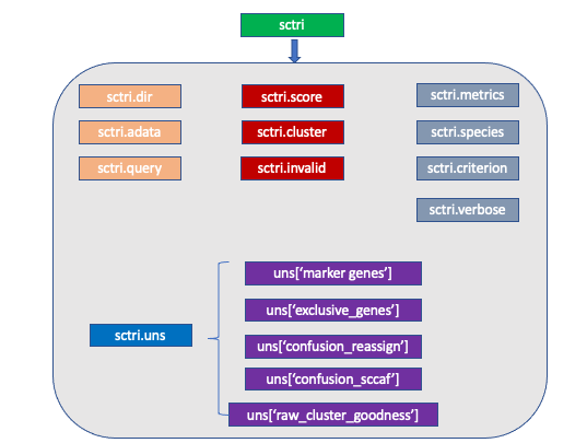
Let’s digest them one by one:
sctri.dir: python string, please specify the path to the folder where all the outputs will fall into.
sctri.adata: AnnData Object, stored the expression values and cell/feature metadata.
sctri.query: python list, each item in the list corresponds to a column name in sctri.adata.obs. Recalling the schema of scTriangualte, please tell
the program what sets of annotations you want to consider. For instance, I want to compare following four annotations:
sctri.query = ['leiden_resolution1','leiden_resolution2','azimuth_mapping_reference1','adt_annotations']
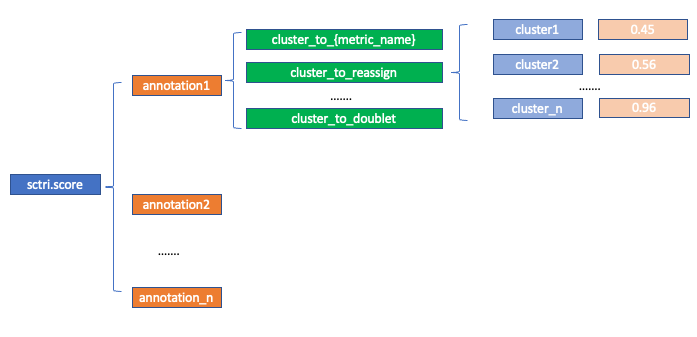
sctri.score: Nested python dictionary (for internal use, users do not need to specify), storing the goodness (measured by each metric) of each cluster in each annotation. The metric corresponds to
self.metrics (see below), the annontation corresponds to self.query. If you want to access:
sctri.score['annotation1']['cluster_to_reassign']['cluster1']
# result will be 0.45
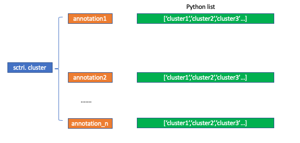
sctri.cluster: Nested python dictionary (for internal use, users do not need to specify), storing the hierarchy of each annotation and cluster name. Likewise,
if you want to access the information:
sctri.cluster['annotation1'][0]
# result will be 'cluster1'
sctri.invalid: Python list, this contains the cluster names (i.e. annotation1@cluster3) that the program labelled as “not stable”. By default, scTriangulate
filters the raw cluster by win_fraction, meaning how many fraction of cells in the original cluster are retained after the “game”. Those invalid cluster will
be excluded from final pruned result, and cells within those invalid clusters will be reassigned to the nearest neighbors. Users can also append cluster name
to the list, by:
sctri.invalid.append('annotation1@cluster3')
# then cells within this cluster will be reassigned in the pruning step.
sctri.metrics: Python list, this contains the metrics we want to use to assess how good a cluster is. By default, the value of this list is:
sctri.metrics = ['reassign','tfidf10','SCCAF','doublet']
which means each cluster will be scanned using these four scores, each score correponds to an underlying function that the program has already implemented, you can add additional metrics by:
sctri.add_new_metrics({'my_metric':callable})
And now the cluster will also be scanned using user defined metric function.
sctri.species: Python string, now only support either “human” or “mouse”. It only affects how the program retrieve the “artifact” genes names in a small
internal database (txt file), including ribosomal genes, mitochondrial genes, etc.
sctri.criterion: Python int, it specify how the program labels “artifact genes”, we assume cellcycle gene, ribosome gene, mitochrondrial gene, antisense,
and predict_gene may not be what the users want, but it varies by the need. So the user can choose from these 6 modes. Genes being labelled as “artifact” will
no longer be considered in the marker genes and downstream assessment:
criterion1: all will be artifact.
criterion2: all will be artifact except cellcycle (default).
criterion3: all will be artifact except cellcycle, ribosome.
criterion4: all will be artifact except cellcycle, ribosome, mitochondrial.
criterion5: all will be artifact except cellcycle, ribosome, mitochondrial, antisense.
criterion6: all will be artifact except cellcycle, ribosome, mitochondrial, antisense, predict_gene.
self.verbose: Python int. 1 means output the log to the stdout, 2 means write to a log file. Default is 1.
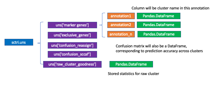
self.uns: Python dictionary, which inspired by scanpy. Here we by default store some very important information including markers genes. To access:
sctri.uns['marker_genes']['anntation1'].loc[:['cluster1','cluster2']]
Visualization
scTriangulate offers a powerful toolkit allowing end users to visualize the hidden heterogeneity in many different ways, also the color Module
provide necessary function to assist in making publication quality figures. Here we highlight some of the plotting function and we would like to refer
the users to the API part for more details.
plot_heterogeneity
This is the main feature of scTriangulate visualizations, built on top of scanpy. Since scTriangualte can mix-and-match cluster boundaries from diverse annotations, it empowers the users to discover further and hidden heterogeneity. Now, question is how the user can visualize the heterogeneity?
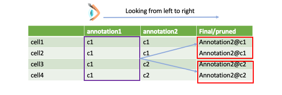
The philosophy behind this function is to first pick a viewpoint from which we want to look at the final result. For instance, here we choose “annotation1” as the viewpoint. As you can see, annoatation@c1 has been suggested to be divided by two sub populations, now we want to know:
how these two sub populations are lait out on umap?
what are the differentially expressed features between these two sub populations?
Let’s show some of the functionalities:
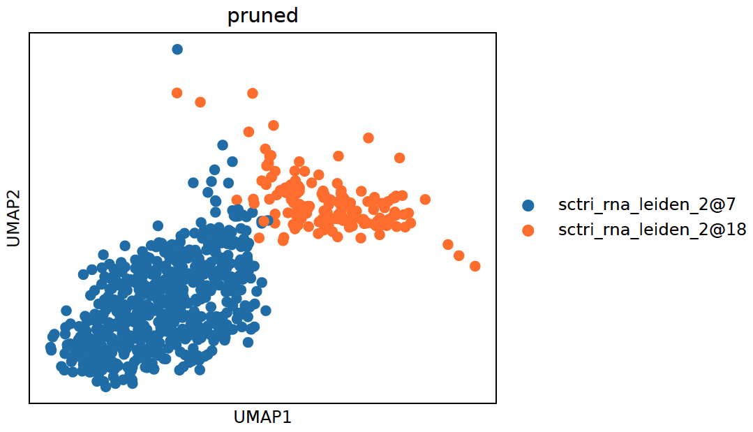
1. UMAP:
sctri.plot_heterogeneity(key='sctri_rna_leiden_1',cluster='6',style='umap')
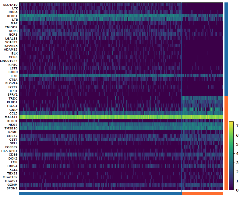
2. Heatmap:
sctri.plot_heterogeneity(key='sctri_rna_leiden_1',cluster='6',style='heatmap')
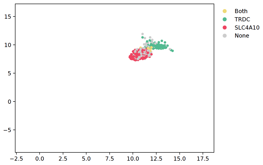
3. dual_gene_plot:
sctri.plot_heterogeneity(key='sctri_rna_leiden_1',cluster='6',style='dual_gene',genes=['TRDC','SLC4A10'])
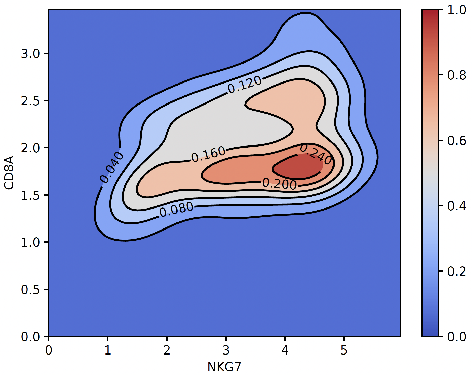
4. coexpression_plot:
sctri.plot_heterogeneity(key='lenden1',cluster='6',style='coexpression',kind='contourf',gene1='NKG7',gene2='CD8A')
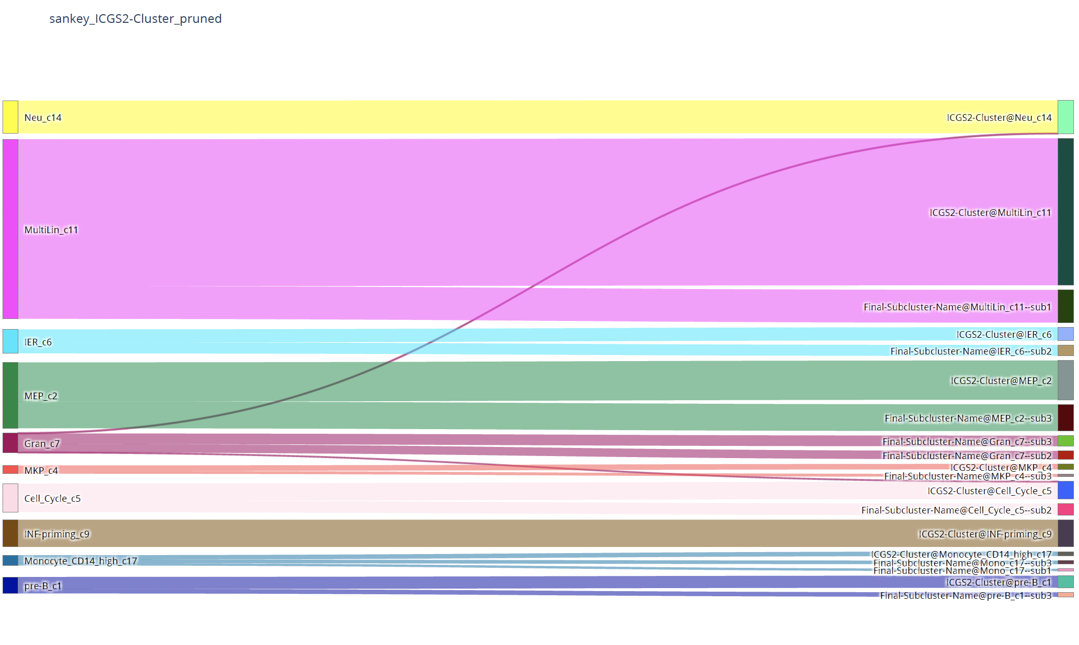
plot_two_column_sankey
To visualize the correspondence of two annotations:
sctri.plot_two_column_sankey('leiden1','leiden2',margin=5)
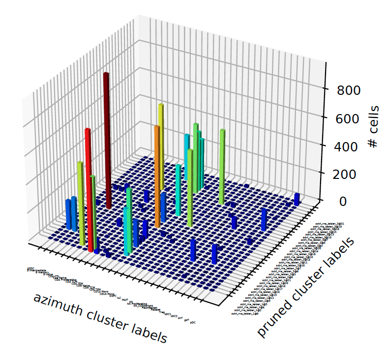
plot_concordance
When we have more than 2 annotation-sets, we want to know how they correspond to each other, what fraction of cells in annotation1 flow into another annotation and vice versus:
sctri.plot_concordance(key1='azimuth',key2='pruned',style='3dbar')
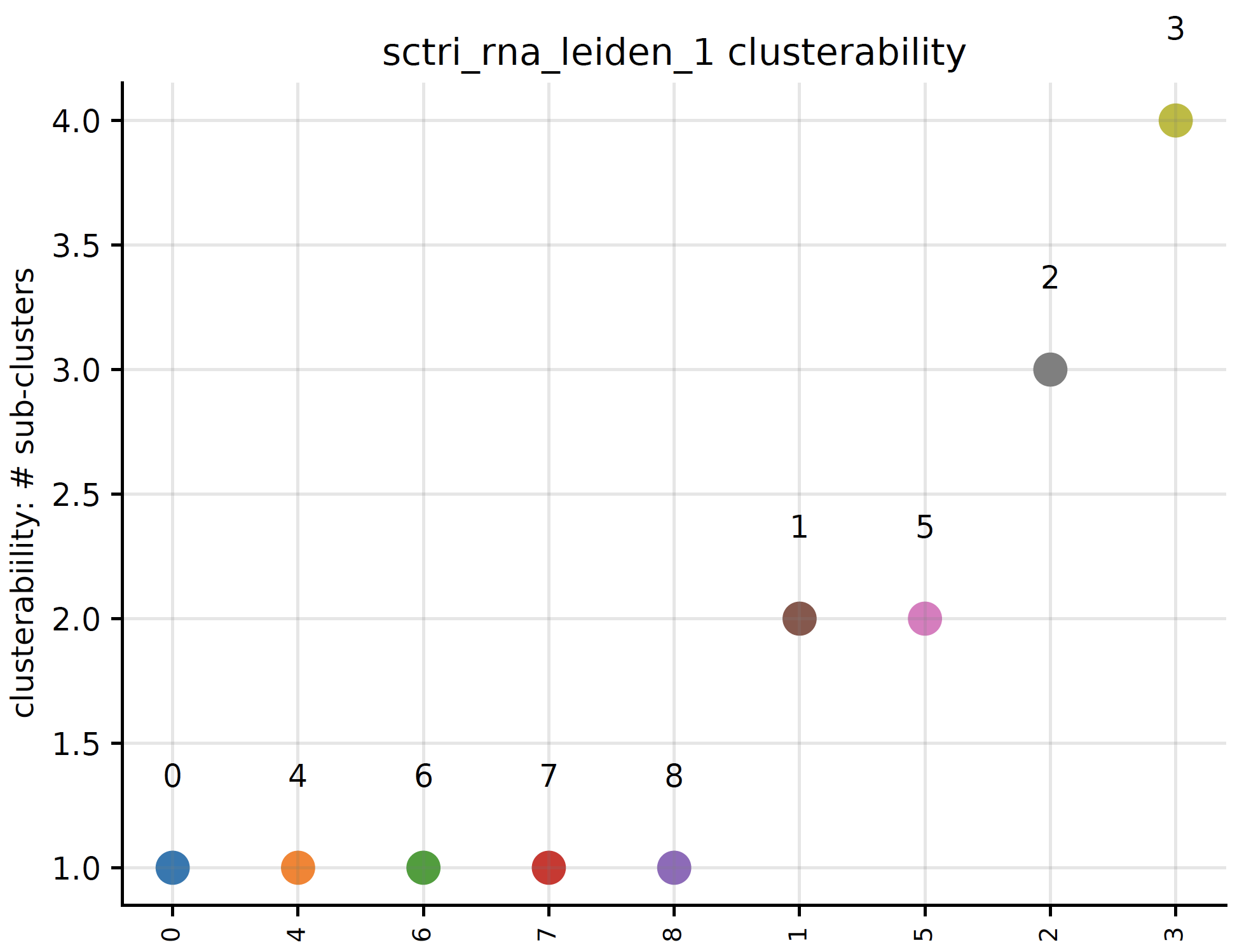
plot_clusterability
Do you want to know for a specific annotation-set, which cluster is most likely to be subdivided and which is the least? We refer to this as clusterability:
sctri.plot_clusterability(key='sctri_rna_leiden_1',col='raw',fontsize=8)
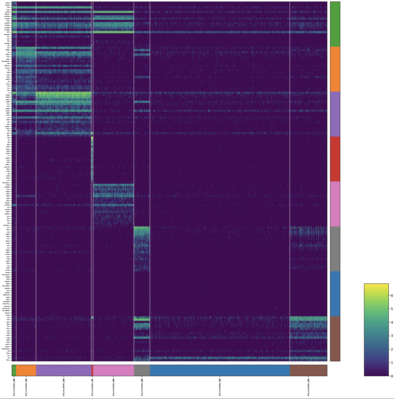
plot_long_heatmap
A heatmap that can be arbitrarily long and ALWAYS display every gene:
sctri.plot_long_umap(n_features=20,figsize=(20,20))
plot_multi_modal_feature_rank
In multi-modal setting, a cluster’s identify usually defined by all modalities, do you want to know by which modality a cluster is mainly defined?:
sctri.plot_multi_modal_feature_rank(cluster='sctri_rna_leiden_2@10')
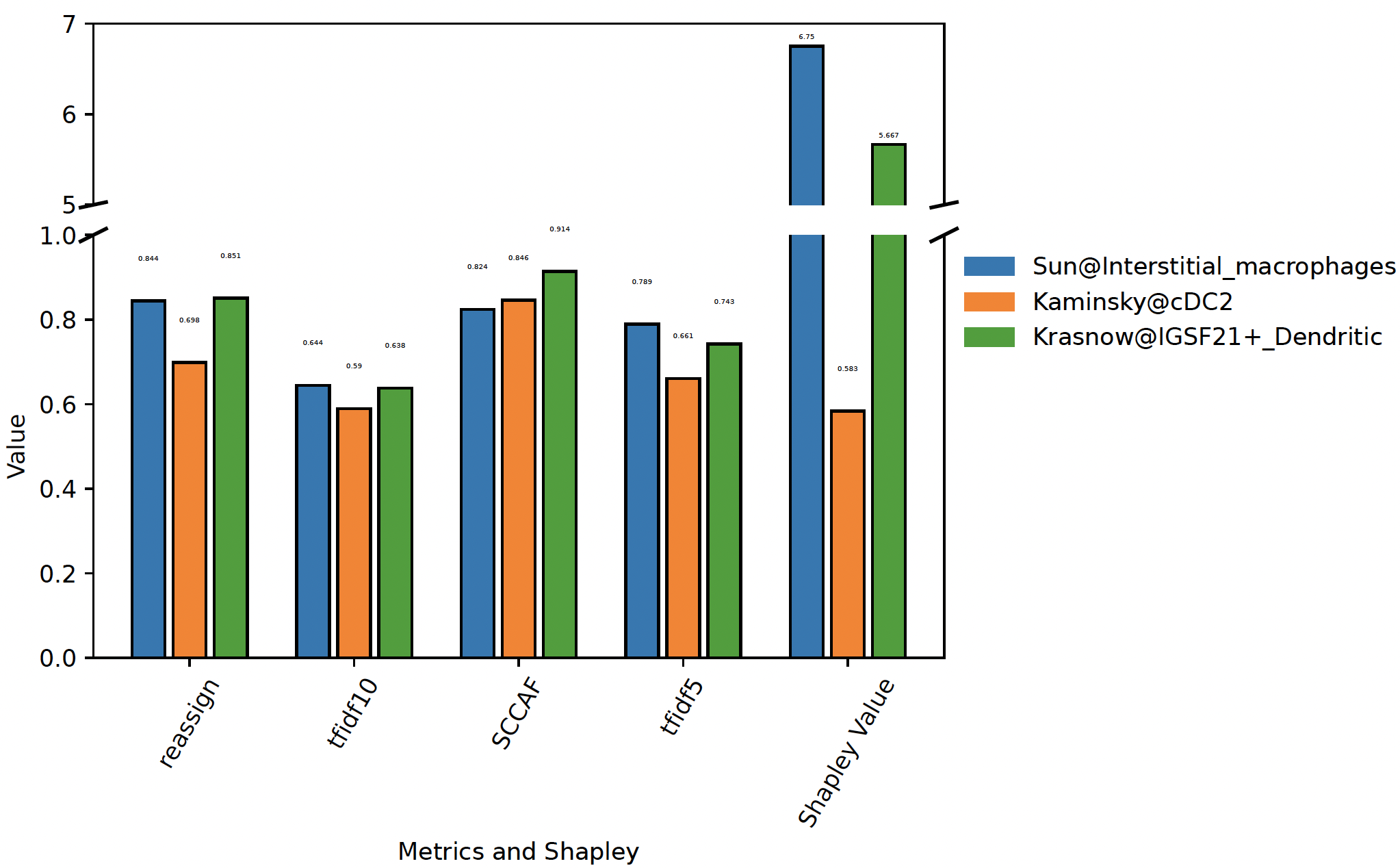
plot_stability
Plot the stability of competing clusters:
sctri.plot_stability(clusters=['Sun@Interstitial_macrophages','Kaminsky@cDC2','Krasnow@IGSF21+_Dendritic'],broke=True,top_ylim=[5,7])
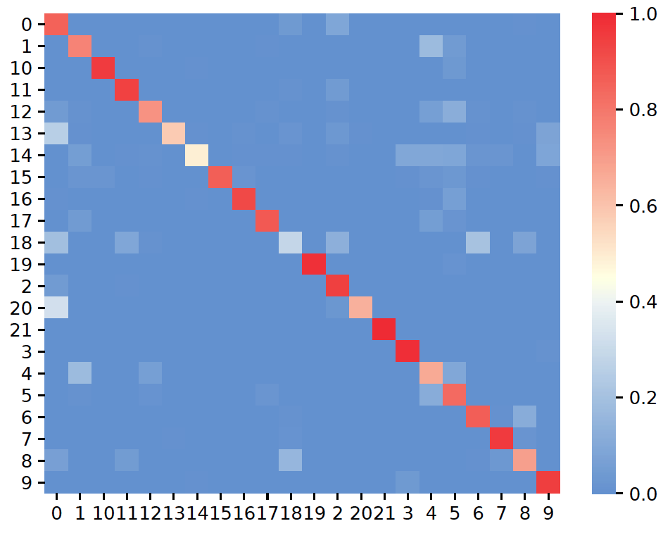
plot_confusion
It allows you to visualize the stability of each clustes in one annotation:
sctri.plot_confusion(name='confusion_reassign',key='sctri_rna_leiden_1')