API

ScTriangulate Class Methods

__init__()

class sctriangulate.main_class.ScTriangulate(dir, adata, query, species='human', criterion=2, verbose=1, reference=None, add_metrics={'tfidf5': <function tf_idf5_for_cluster>}, predict_doublet=False)

How to create/instantiate ScTriangulate object.

Parameters

• dir – Output folder path on the disk, will create if not exist

• adata – input adata file

• query – a python list contains the annotation names to query

• species – string, either human (default) or mouse, it will impact how the program searches for artifact genes in the database

• criterion –

  int, it controls what genes would be considered as artifact genes:

  • criterion1: all will be artifact

  • criterion2: all will be artifact except cellcycle [Default]

  • criterion3: all will be artifact except cellcycle, ribosome

  • criterion4: all will be artifact except cellcycle, ribosome, mitochondrial

  • criterion5: all will be artifact except cellcycle, ribosome, mitochondrial, antisense

  • criterion6: all will be artifact except cellcycle, ribosome, mitochondrial, antisense, predict_gene

• verbose – int, it controls how the log file will be generated. 1 means print to stdout (default), 2 means print to a file in the directory specified by dir parameter.

• add_metrics – python dictionary. These allows users to add additional metrics to favor or disqualify certain cluster. By default, we add tfidf5 score {‘tfidf5’:tf_idf5_for_cluster}, remember the value in the dictionary should be the name of a callable, user can define the callable by themselves. If don’t want any addded metrics, using empty dict {}.

• predict_doublet –

  boolean or string, whether to predict doublet using scrublet or not. Valid value:

  • True: will predict doublet score

  • False: will not predict doublet score

  • (string) precomputed: will not predict doublet score but just use existing one

Note

For the callable, the signature should be func(adata,key,**kwargs) -> mapping {cluster1:0.5,cluster2:0.6}, when running the program in lazy_run function, we need to specify added_metrics_kwargs as a list, each element in the list is a dictionary that corresponds to the kwargs that will be passed to each callable.

Example:

adata = sc.read('pbmc3k_azimuth_umap.h5ad')
sctri = ScTriangulate(dir='./output',adata=adata,query=['leiden1','leiden2','leiden3'])

(statis) deserialize()

sctriangulate.main_class.ScTriangulate.deserialize(name)

This is static method, to deserialize a pickle file on the disk back to the ram as a sctri object

Parameters

name – string, the name of the pickle file on the disk.

Examples:

ScTriangulate.deserialize(name='after_rank_pruning.p')

(statics) salvage_run()

sctriangulate.main_class.ScTriangulate.salvage_run(step_to_start, last_step_file, outdir=None, scale_sccaf=True, layer=None, added_metrics_kwargs=[{'species': 'human', 'criterion': 2, 'layer': None}], compute_shapley_parallel=True, shapley_mode='shapley_all_or_none', shapley_bonus=0.01, win_fraction_cutoff=0.25, reassign_abs_thresh=10, assess_raw=False, assess_pruned=True, viewer_cluster=True, viewer_cluster_keys=None, viewer_heterogeneity=True, viewer_heterogeneity_keys=None, nca_embed=False, n_top_genes=3000, other_umap=None, heatmap_scale=None, heatmap_cmap='viridis', heatmap_regex=None, heatmap_direction='include', heatmap_n_genes=None, heatmap_cbar_scale=None)

This is a static method, which allows to user to resume running scTriangulate from certain point, instead of running from very beginning if the intermediate files are present and intact.

Parameters

• step_to_start – string, now support ‘assess_pruned’.

• last_step_file – string, the path to the intermediate from which we start the salvage run.

• outdir – None or string, whether to change the outdir or not.

Other parameters are the same as lazy_run function.

Examples:

ScTriangulate.salvage_run(step_to_start='assess_pruned',last_step_file='output/after_rank_pruning.p')

add_new_metrics()

sctriangulate.main_class.ScTriangulate.add_new_metrics(self, add_metrics)

Users can add new callable or pre-implemented function to the sctri.metrics attribute.

Parameters

add_metrics – dictionary like {‘metric_name’: callable}, the callable can be a string of a scTriangulate pre-implemented function, for example, ‘tfidf5’,’tfidf1’. Or a callable.

Examples:

sctri.add_new_metrics(add_metrics={'tfidf1':tfidf1})  # make sure first from sctriangualte.metrics import tfidf1

add_to_invalid()

sctriangulate.main_class.ScTriangulate.add_to_invalid(self, invalid)

add individual raw cluster names to the sctri.invalid attribute list.

Parameters

invalid – list or string, contains the raw cluster names to add

Examples:

sctri.add_to_invalid(invalid=['annotation1@c3','annotation2@4'])
sctri.add_to_invalid(invalid='annotation1@3')

add_to_invalid_by_win_fraction()

sctriangulate.main_class.ScTriangulate.add_to_invalid_by_win_fraction(self, percent=0.25)

add individual raw cluster names to the sctri.invalid attribute list by win_fraction

Parameters

percent – float, from 0-1, the fraction of cells within a cluster that were kept after the game. Default: 0.25

Examples:

sctri.add_to_invalid_by_win_fraction(percent=0.25)

clear_invalid()

sctriangulate.main_class.ScTriangulate.clear_invalid(self)

reset/clear the sctri.invalid to an empty list

Examples:

sctri.clear_invalid()

cluster_performance()

sctriangulate.main_class.ScTriangulate.cluster_performance(self, cluster, competitors, reference, show_cluster_number=False, metrics=None, ylim=None, save=True, format='pdf')

automatic benchmark of scTriangulate clusters with all the individual or competitor annotation, against a ‘gold standard’ annotation, measured by all unsupervised cluster metrics (homogeneity, completeness, v_measure, ARI, NMI).

Parameters

• cluster – string, the scTriangulate annotation column name, for example, pruned

• competitiors – list of string, each is a column name of a competitor annotation

• reference – string, the column name containing reference annotation, for example, azimuth

• show_cluster_number – bool, whether to show the number of cluster of each annotation in the performance line plot

• metrics – None or any other, if not None, ARI and NMI will also be plotted

• ylim – None or a tuple, specifiying the ylims of plot

• save – bool, whether to save the figure

• format – string, default is pdf, the format to save

Examples:

sctri.cluster_performance(cluster='pruned',competitors=['sctri_rna_leiden_1','sctri_rna_leiden_2','sctri_rna_leiden_3'],
                          reference='azimuth',show_cluster_number=True,metrics=None)

compute_metrics()

sctriangulate.main_class.ScTriangulate.compute_metrics(self, parallel=True, scale_sccaf=False, layer=None, added_metrics_kwargs=[{'species': 'human', 'criterion': 2, 'layer': None}], cores=None)

main function for computing the metrics (defined by self.metrics) of each clusters in each annotation. After the run, q (# query) * m (# metrics) columns will be added to the adata.obs, the column like will be like {metric_name}@{query_annotation_name}, i.e. reassign@sctri_rna_leiden_1

Parameters

• parallel – boolean, whether to run in parallel. Since computing metrics for each query annotation is idependent, the program will automatically employ q (# query) cores under the hood. If you want to fully leverage this feature, please make sure you specify at least q (# query) cores when running the program. It is highly recommend to run this in parallel. However, when the dataset is super large and have > 10 query annotation, we may encounter RAM overhead, in this case, sequential mode will be needed. Default: True

• scale_sccaf – boolean, when running SCCAF score, since it is a logistic regression problem at its core, this parameter controls whether scale the expression data or not. It is recommended to scale the data for any machine learning algorithm, however, the liblinaer solver has been demonstrated to be robust to the scale/unscale options. When the dataset > 50,000 cells or features > 1000000 (ATAC peaks), it is advised to not scale it for faster running time.

• layer – None or str, the adata layer where the raw count is stored, useful when calculating tfidf score when adata.X has been skewed (no zero value, like totalVI denoised value)

• added_metrics_kwargs – list, see the notes in __init__ function, this is to specify additional arguments that will be passed to each added metrics callable.

• cores – None or int, how many cores you’d like to specify, by default, it is min(n_annotations,n_available_cores) for metrics computing, and n_available_cores for other parallelizable operations

Examples:

sctri.compute_metrics(parallel=False)

compute_shapley()

sctriangulate.main_class.ScTriangulate.compute_shapley(self, parallel=True, mode='shapley_all_or_none', bonus=0.01, cores=None)

Main core function, after obtaining the metrics for each cluster. For each single cell, let’s calculate the shapley value for each annotation and assign the cluster to the one with highest shapley value.

Parameters

• parallel – boolean. Whether to run it in parallel. (scatter and gather). Default: True

• mode –

  string, accepted values:

  • shapley_all_or_none: default, computing shapley, and players only get points when it beats all

  • shapley: computing shapley, but players get points based on explicit ranking, say 3 players, if ranked first, you get 3, if running up, you get 2

  • rank_all_or_none: no shapley computing, importance based on ranking, and players only get points when it beats all

  • rank: no shapley computing, importance based on ranking, but players get points based on explicit ranking as described above

• bonus – float, default is 0.01, an offset value so that if the runner up is just {bonus} inferior to first place, it will still be a valid cluster

• cores – None or int, None will run mp.cpu_counts() to get all available cpus.

Examples:

sctri.compute_shapley(parallel=True)

confusion_to_df()

sctriangulate.main_class.ScTriangulate.confusion_to_df(self, mode, key)

Print out the confusion matrix with cluster labels (dataframe).

Parameters

• mode – either ‘confusion_reassign’ or ‘confusion_sccaf’

• mode – python string, for example, ‘annotation1’

Examples:

sctri.confusion_to_df(mode='confusion_reassign',key='annotation1')

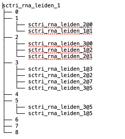
display_hierarchy()

sctriangulate.main_class.ScTriangulate.display_hierarchy(self, ref_col, query_col, save=True)

Display the hierarchy of suggestive sub-clusterings, see the example results down the page.

Parameters

• ref_col – string, the annotation/column name in adata.obs which we want to inspect how it can be sub-divided

• query_col – string, any cluster annotation column name

• save – boolean, whether to save it to a file or stdout. Default: True

Examples:

sctri.display_hierarchy(ref_col='sctri_rna_leiden_1',query_col='raw')

doublet_predict()

sctriangulate.main_class.ScTriangulate.doublet_predict(self)

wrapper function of running scrublet, will add a column on adata.obs called ‘doublet_scores’

Examples:

sctri.doublet_predict()

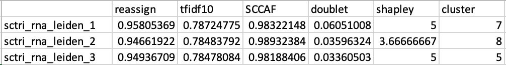
elo_rating_like()

sctriangulate.main_class.ScTriangulate.elo_rating_like(self)

Computing an overall quality score for each annotation, like the idea of Elo Rating in chess in which it can reflect the probability that one player will win in a chess match. Here, we argue the overall quality score should be defined by the average of all cells’ shapley value in all clusters, normalized by the number of players (annotation), and further normalized by number of clusters, as our computation of shapley is an additive process such that more player will result in higher shapley value. This step should be run after shapley value were evaluated.

Return result_dic

a dictionary keyed by annotation, value is overall quality score

Examples:

result_dic = sctri.elo_rating_like()

# {'sctri_rna_leiden_1': 1.5053613872472829, 'sctri_rna_leiden_2': 1.0973714905049967, 'sctri_rna_leiden_3': 1.1032324231884296}

extract_stability()

sctriangulate.main_class.ScTriangulate.extract_stability(self, keys=None)

To extract cluster stability information

Params keys

a list, containing the annotation column names, None means all in self.query

Examples:

sctri.extract_stability(keys=['annotation1','annotation2'])

gene_to_df()

sctriangulate.main_class.ScTriangulate.gene_to_df(self, mode, key, raw=False, col='purify', n=100)

Output {mode} genes for all clusters in one annotation (key), mode can be either ‘marker_genes’ or ‘exclusive_genes’.

Parameters

• mode – python string, either ‘marker_genes’ or ‘exclusive_genes’

• key – python string, annotation name

• raw – False will generate non-raw (human readable) format. Default: False

• col – Only when mode==’marker_genes’, whether output ‘whole’ column or ‘purify’ column. Default: purify

• n – Only when mode==’exclusive_genes’, how many top exclusively expressed genes will be printed for each cluster.

Examples:

sctri.gene_to_df(mode='marker_genes',key='annotation1')
sctri.gene_to_df(mode='exclusive_genes',key='annotation1')

get_metrics_and_shapley()

sctriangulate.main_class.ScTriangulate.get_metrics_and_shapley(self, barcode, save=True)

For one single cell, given barcode/or other unique index, generate the all conflicting cluster from each annotation, along with the metrics associated with each cluster, including shapley value.

Parameters

• barcode – string, the barcode for the cell you want to query.

• save – save the returned dataframe to directory or not. Default: True

Returns

DataFrame

Examples:

sctri.get_metrics_and_shapley(barcode='AAACCCACATCCAATG-1',save=True)

lazy_run()

sctriangulate.main_class.ScTriangulate.lazy_run(self, compute_metrics_parallel=True, scale_sccaf=False, layer=None, cores=None, added_metrics_kwargs=[{'species': 'human', 'criterion': 2, 'layer': None}], compute_shapley_parallel=True, shapley_mode=None, shapley_bonus=0.01, win_fraction_cutoff=0.25, reassign_abs_thresh=10, assess_raw=False, assess_pruned=False, viewer_cluster=False, viewer_cluster_keys=None, viewer_heterogeneity=False, viewer_heterogeneity_keys=None, nca_embed=False, n_top_genes=3000, other_umap=None, heatmap_scale=None, heatmap_cmap='viridis', heatmap_regex=None, heatmap_direction='include', heatmap_n_genes=None, heatmap_cbar_scale=None)

This is the highest level wrapper function for running every step in one goal.

Parameters

• compute_metrics_parallel – boolean, whether to parallelize compute_metrics step. Default: True

• scale_sccaf – boolean, whether to first scale the expression matrix before running sccaf score. Default: False

• layer – None or str, the adata layer where the raw count is stored, useful when calculating tfidf score when adata.X has been skewed (no zero value, like totalVI denoised value)

• cores – None or int, how many cores you’d like to specify, by default, it is min(n_annotations,n_available_cores) for metrics computing, and n_available_cores for other parallelizable operations

• added_metrics_kwargs – list, see the notes in __init__ function, this is to specify additional arguments that will be passed to each added metrics callable.

• compute_shapley_parallel – boolean, whether to parallelize compute_parallel step. Default: True

• shapley_mode –

  string, accepted values:

  • shapley_all_or_none: computing shapley, and players only get points when it beats all

  • shapley: computing shapley, but players get points based on explicit ranking, say 3 players, if ranked first, you get 3, if running up, you get 2

  • rank_all_or_none: no shapley computing, importance based on ranking, and players only get points when it beats all

  • rank: no shapley computing, importance based on ranking, but players get points based on explicit ranking as described above

  • None: if n_annotations <= 15, use shapley_all_or_none, if n_anntations > 15, use rank

• shapley_bonus – float, default is 0.01, an offset value so that if the runner up is just {bonus} inferior to first place, it will still be a valid cluster

• win_fraction_cutoff – float, between 0-1, the cutoff for function add_invalid_by_win_fraction. Default: 0.25

• reassign_abs_thresh – int, the cutoff for minimum number of cells a valid cluster should haves. Default: 10

• assess_raw – boolean, whether to run the same cluster assessment metrics on raw cluster labels. Default: False

• assess_pruned – boolean, whether to run same cluster assessment metrics on final pruned cluster labels. Default: False

• viewer_cluster – boolean, whether to build viewer html page for all clusters’ diagnostic information. Default: False

• viewer_cluster_keys – list, clusters from what annotations we want to view on the viewer, only clusters within this annotation whose diagnostic plot will be generated under the dir name figure4viewer. Default: None, means all annotations in the sctri.query will be used.

• viewer_heterogeneity – boolean, whether to build the viewer to show the heterogeneity based on one reference annotation. Default: False

• viewer_heterogeneity_keys – list, the annotations we want to serve as the reference. Default: None, means the first annotation in sctri.query will be used as the reference.

Examples:

sctri.lazy_run(viewer_heterogeneity_keys=['annotation1','annotation2'])

modality_contributions()

sctriangulate.main_class.ScTriangulate.modality_contributions(self, mode='marker_genes', key='pruned', tops=20, regex_dict={'adt': '^AB_', 'atac': '^chr\\d{1,2}'})

calculate the modality contributions for multi modal analysis, the modality contributions of each modality of each cluster means the number of features from this modality that made into the top {tops} feature list. Multiple columns will be added to obs, they are corresponding to the number of modalities considered

Parameters

• mode – string, either ‘marker_genes’ or ‘exclusive_genes’.

• key – string, any valid categorical column in self.adata.obs

• tops – int, the top n features to consider for each cluster.

• regex_dict – dict, keyed by modality name, value is a raw string representing the regex pattern for parsing each modality features

Examples:

sctri.modality_contributions(mode='marker_genes',key='pruned',tops=20)

penalize_artifact()

sctriangulate.main_class.ScTriangulate.penalize_artifact(self, mode, stamps=None, parallel=True)

An optional step after running compute_metrics step and before the compute_shapley step. Basically, we penalize clusters with certain properties by set all their metrics to zero, which forbid them to win in the following “game” step. These undesirable properties can be versatial, for example, cellcylce gene enrichment. We current support two mode:

1. mode1: void, users specifiy which cluster they want to penalize via stamps parameter.

2. mode2: cellcycle, program automatically label clusters whose gsea_hit > 5 and gsea_score > 0.8 as invalid cellcyle enriched clusters. And those clusters will be penalized.

Parameters

• mode – string, either ‘void’ or ‘cellcycle’.

• stamps – list, contains cluster names that the users want to penalize.

• parallel – boolean, whether to run this in parallel (scatter and gather). Default: True.

Examples:

sctri.penalize_artifact(mode='void',stamps=['sctri_rna_leiden_1@c3','sctri_rna_leiden_2@c5'])
sctri.penalize_artifact(mode='cellcyle')

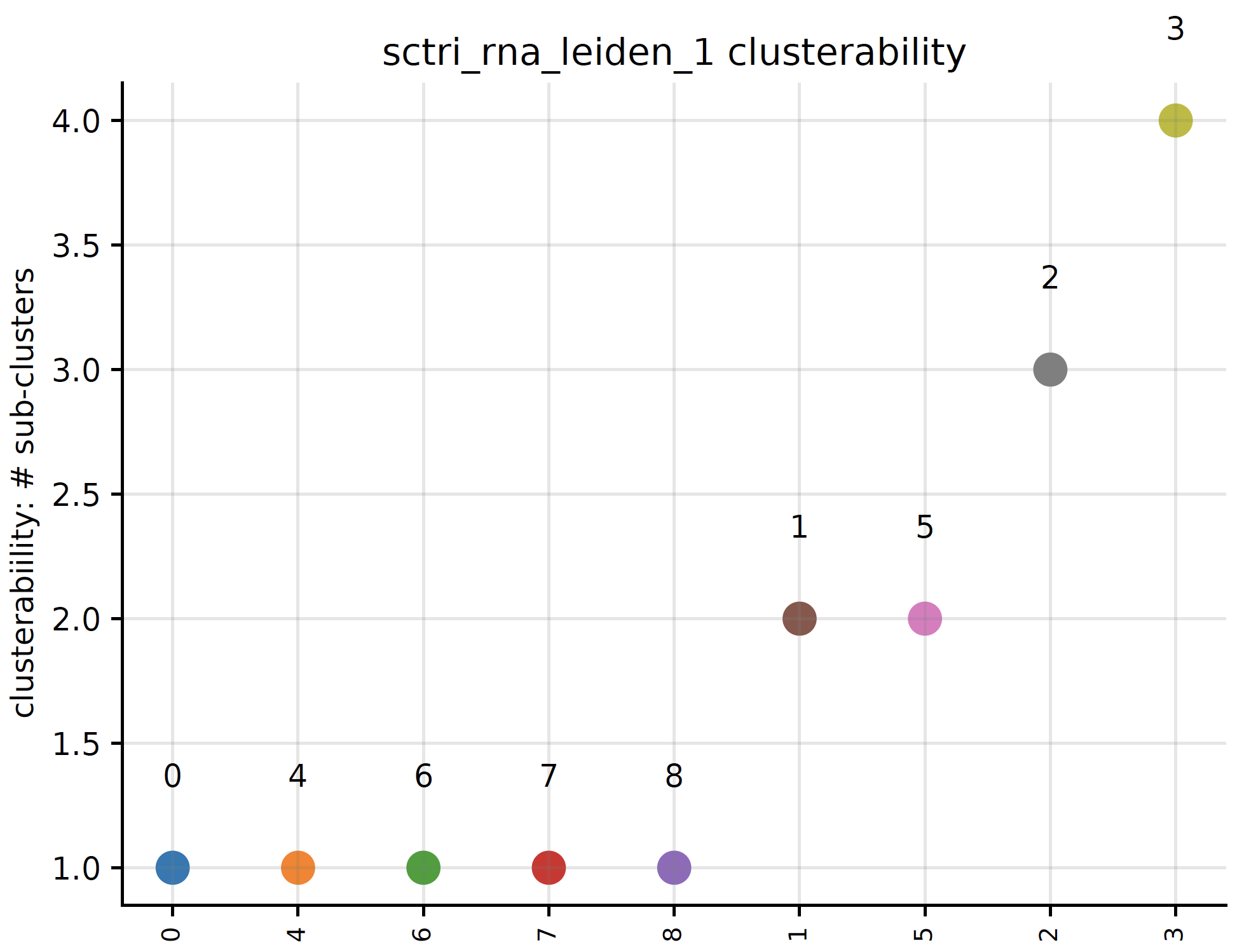
plot_clusterability()

sctriangulate.main_class.ScTriangulate.plot_clusterability(self, key, col, fontsize=3, plot=True, save=True)

We define clusterability as the number of sub-clusters the program finds out. If a cluster has being suggested to be divided into three smaller clusters, then the clueterability of this cluster will be 3.

Parameters

• key – string. The clusters from which annotation that you want to assess clusterability.

• col – string. Either ‘raw’ cluster or ‘pruned’ cluster.

• fontsize – int. The fontsize of x-ticklabels. Default: 3

• plot – boolean. Whether to plot the scatterplot or not. Default : True.

• save – boolean. Whether to save the plot or not. Default: True

Returns

python dictionary. {cluster1:#sub-clusters}

Examples:

sctri.plot_clusterability(key='sctri_rna_leiden_1',col='raw',fontsize=8)

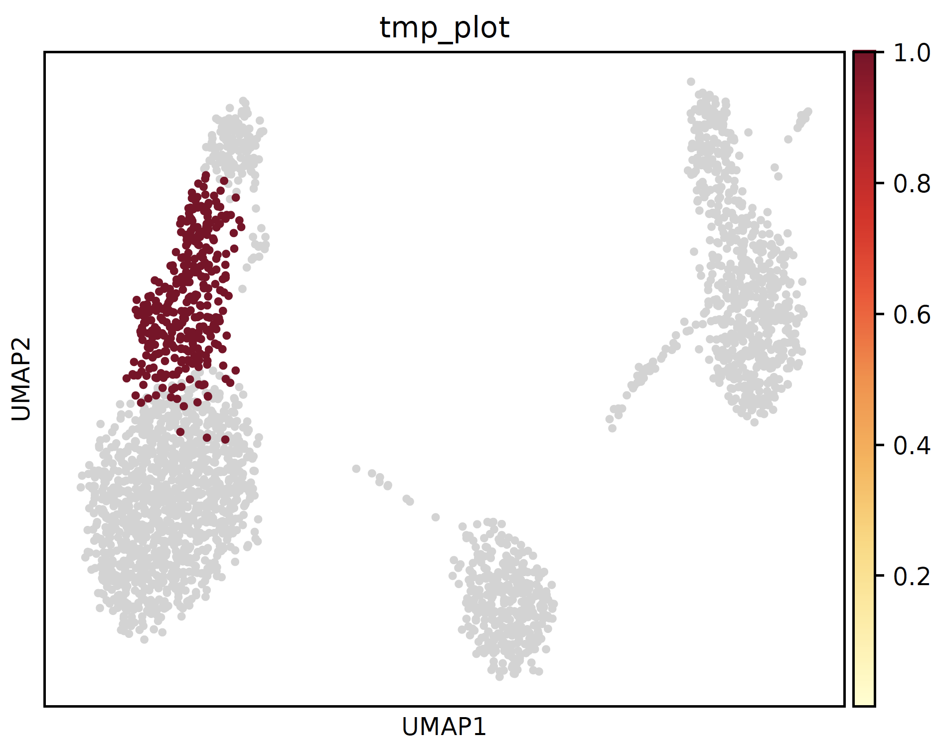
plot_cluster_feature()

sctriangulate.main_class.ScTriangulate.plot_cluster_feature(self, key, cluster, feature, enrichment_type='enrichr', save=True, format='pdf')

plot the feature of each single clusters, including:

1. enrichment of artifact genes

2. marker genes umap

3. exclusive genes umap

4. location of clutser umap

Parameters

• key – string. Name of the annation.

• cluster – string. Name of the cluster in the annotation.

• feature – string, valid value: ‘enrichment’,’marker_genes’, ‘exclusive_genes’, ‘location’

• enrichmen_type – string, either ‘enrichr’ or ‘gsea’.

• save – boolean, whether to save the figure.

• format – string, which format for the saved figure.

Example:

sctri.plot_cluster_feature(key='sctri_rna_leiden_1',cluster='3',feature='enrichment')

Example:

sctri.plot_cluster_feature(key='sctri_rna_leiden_1',cluster='3',feature='marker_genes')

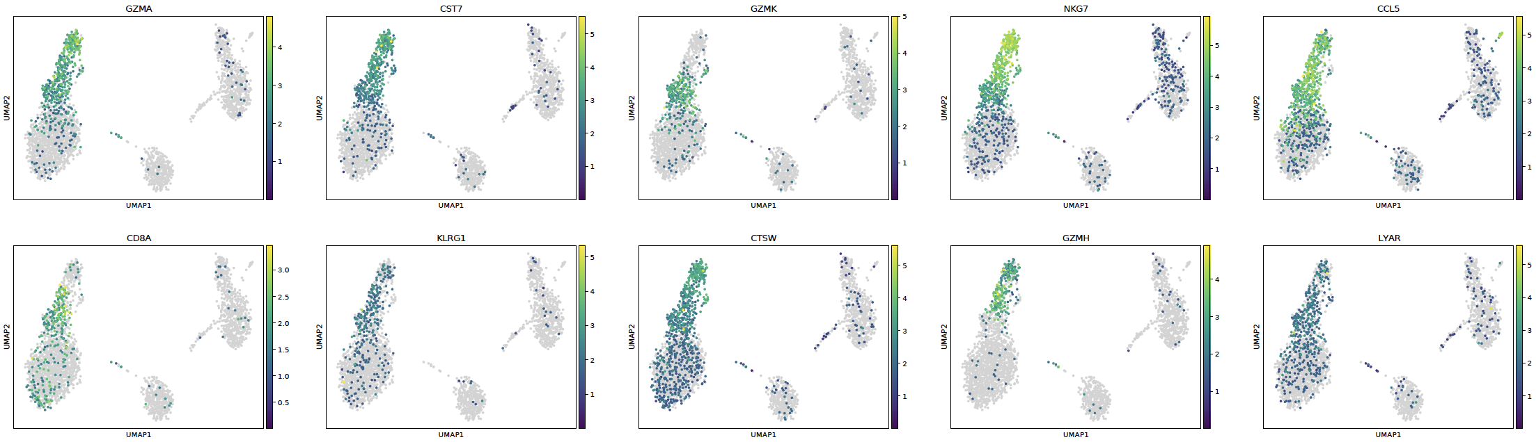
Example:

sctri.plot_cluster_feature(key='sctri_rna_leiden_1',cluster='3',feature='location')

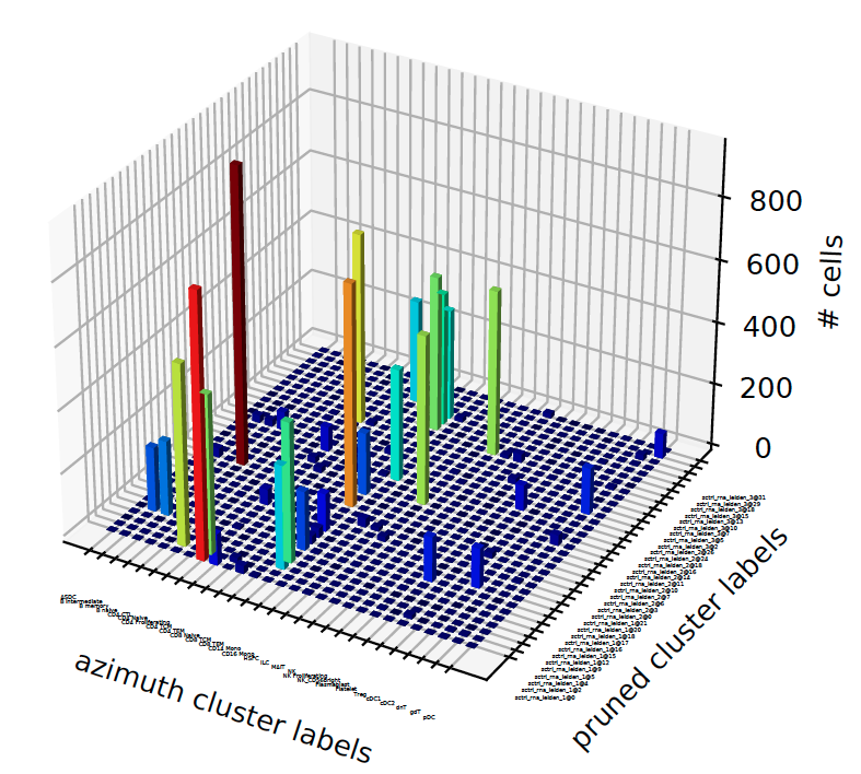
plot_concordance()

sctriangulate.main_class.ScTriangulate.plot_concordance(self, key1, key2, style='3dbar', save=True, format='pdf', cmap=<matplotlib.colors.LinearSegmentedColormap object>, **kwargs)

given two annotation, we want to know how the cluster labels from one correponds to the other.

Parameters

• key1 – string, first annotation key

• key2 – string, second annotation key

• style – string, which style of plot, either ‘heatmap’ or ‘3dbar’

• save – boolean, save the figure or not

• format – string, format to save

• cmap – string or cmap object, the cmap to use for heatmap

Returns

dataframe, the confusion matrix

Examples:

sctri.plot_concordance(key1='azimuth',key2='pruned',style='3dbar')

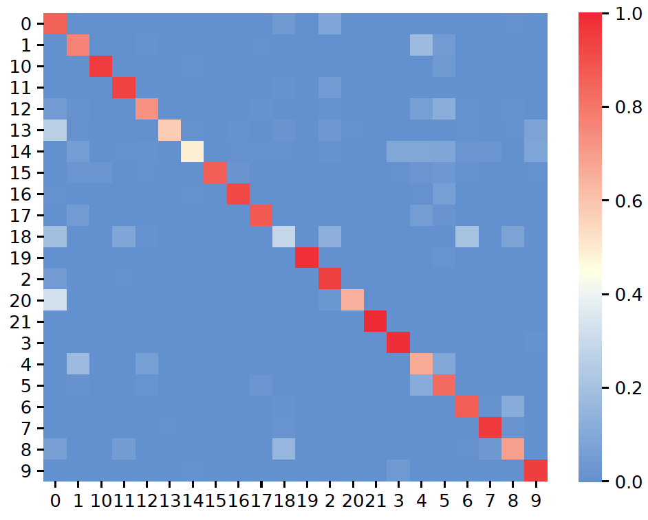
plot_confusion()

sctriangulate.main_class.ScTriangulate.plot_confusion(self, name, key, save=True, format='pdf', cmap=<matplotlib.colors.LinearSegmentedColormap object>, labelsize=None, **kwargs)

plot the confusion as a heatmap.

Parameters

• name – string, either ‘confusion_reassign’ or ‘confusion_sccaf’.

• key – string, a annotation name which we want to assess the confusion matrix of the clusters.

• save – boolean, whether to save the figure. Default: True.

• format – boolean, file format to save. Default: ‘.pdf’.

• cmap – colormap object, Default: scphere_cmap, which defined in colors module.

• labelsize – float, this can adjust the label size on yaxis and xaxis for the resultant heatmap

• kwargs – additional keyword arguments to sns.heatmap().

Examples:

sctri.plot_confusion(name='confusion_reassign',key='sctri_rna_leiden_1')

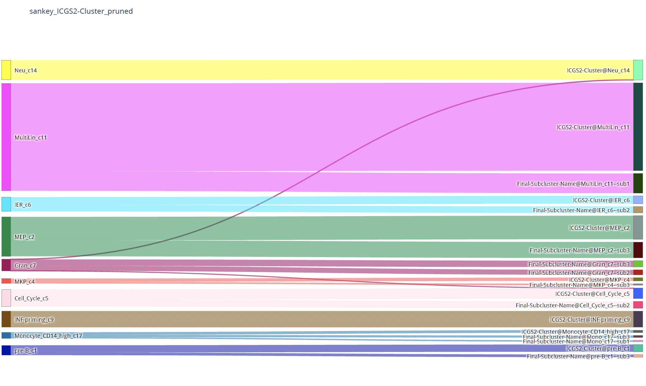
plot_heterogeneity()

sctriangulate.main_class.ScTriangulate.plot_heterogeneity(self, key, cluster, style, col='pruned', save=True, format='pdf', genes=None, umap_zoom_out=True, umap_dot_size=None, subset=None, marker_gene_dict=None, jitter=True, rotation=60, single_gene=None, dual_gene=None, multi_gene=None, merge=None, to_sinto=False, to_samtools=False, cmap='YlOrRd', heatmap_cmap='viridis', heatmap_scale=None, heatmap_regex=None, heatmap_direction='include', heatmap_n_genes=None, heatmap_cbar_scale=None, gene1=None, gene2=None, kind=None, hist2d_bins=50, hist2d_cmap=<matplotlib.colors.ListedColormap object>, hist2d_vmin=1e-05, hist2d_vmax=None, scatter_dot_color='blue', contour_cmap='viridis', contour_levels=None, contour_scatter=True, contour_scatter_dot_size=5, contour_train_kde='valid', surface3d_cmap='coolwarm', **kwarg)

Core plotting function in scTriangulate.

Parameters

• key – string, the name of the annotation.

• cluster – string, the name of the cluster.

• stype –

  string, valid values are as below:

  • umap: plot the umap of this cluster (including its location and its suggestive heterogeneity)

  • heatmap: plot the heatmap of the differentially expressed features across all sub-populations within this cluster.

  • build: plot both the umap and heatmap, benefit is the column and raw colorbar of the heatmap is consistent with the umap color

  • heatmap_custom_gene, plot the heatmap, but with user-defined gene dictionary.

  • heatmap+umap, it is the umap + heatmap_custom_gene, and the colorbars are matching

  • violin: plot the violin plot of the specified genes across sub populations.

  • single_gene: plot the gradient of single genes across the cluster.

  • dual_gene: plot the dual-gene plot of two genes across the cluster, usually these two genes should correspond to the marker genes in two of the sub-populations.

  • multi_gene: plot the multi-gene plot of multiple genes across the cluster.

  • cellxgene: output the h5ad object which are readily transferrable to cellxgene. It also support atac pseudobuld analysis with to_sinto or to_samtools arguments.

  • sankey: plot the sankey plot showing fraction/percentage of cells that flow into each sub population, requiring plotly if you only need html, and kaleido if you need static plot, otherwise, a less pretty matplotlib sankey will be plotted

  • coexpression: visualize the coexpression pattern of two features, using contour plot or hist2d

• col – string, either ‘raw’ or ‘pruned’.

• save – boolean, whether to save or not.

• foramt – string, which format to save.

• genes – list, for violin plot.

• umap_zoom_out – boolean, for the umap, whether to zoom out meaning the scale is the same of the whole umap. Zoom in means an amplified version of this cluster.

• umap_dot_size – int/float, for the umap.

• subset – list, the sub populations we want to keep for plotting.

• marker_gene_dict – dict. The custom genes we want the heatmap to display.

• jitter – float, for the violin plot.

• rotation – int/float, for the violin plot. rotation of the text. Default: 60

• single_gene – string, the gene name for single gene plot

• dual_gene – list, the dual genes for dual gene plot.

• multi_genes – list, the multiple genes for multi gene plot.

• merge – nested list, the sub-populations that we want to merge. [(‘sub-c1’,’sub-c2’),(‘sub-c3’,’sub-c4’)]

• to_sinto – boolean, for cellxgene mode, output the txt files for running sinto to generate pseudobulk bam files.

• to_samtools – boolean,for cellxgene mode, output the txt files for running samtools to generate the pseudobulk bam files.

• cmap – a valid string for matplotlib cmap or scTriangulate color module retrieve_pretty_cmap function return object, default is ‘YlOrRd’, will be used for umap

The following will be used for heatmap only:

Parameters

• heatmap_cmap – a valid string for matplotlib cmap or scTriangulate color module retrieve_pretty_cmap function return object, default is ‘viridis’.

• heatmap_scale –

  None, minmax, median, mean, z_score, default is None, useful when very large or small values exist in the adata.X, scaling can yield better visual effects

  • None means no scale will be performed, the raw valus shown in adata.X will be plotted in the heatmap

  • minmax means the raw values will be row-scaled to [0,1] using a MinMaxScaler

  • median means the raw values will be row-scaled via substracting by the median per row

  • mean means the raw values will be row-scaled via substracting by the mean per row

  • z_score means the raw values will be row-scaled via Scaling (mean-centered and variance normalized)

• heatmap_regex – None or a raw string for example r’^AB_’ (meaning selecing all ADT features as scTriangulate by default prefix ADT features will AB_), the usage of that is to only display certain features from certain modlaities. The underlying implementation is just a regular expression selection.

• heatmap_direction – string, ‘include’ or ‘exclude’, it is along with the heatmap_regex parameter, include means doing positive selection, exclude means to exclude the features that match with the heatmap_regex

• heatmap_n_genes – an integer, by default, program display 50//n_cluster genes for each cluster, this will overwrite the default.

• heatmap_cbar_scale – None or a tuple or a fraction. A tuple for example (-0.5,0.5) will clip the colorbar within -0.5 to 0.5, a fraction number for instance 0.25, will shrink the default colorbar range say -1 to 1 to -0.25 to 0.25

The following will be used for coexpression plot only:

Parameters

• gene1 – the first gene/features to inspect, the gene name, a string.

• gene2 – the second gene/features to inspect, the gene name, a string.

• kind – a string, ‘scatter’ or ‘hist2d’ or ‘contour’ or ‘contourf’ or ‘surface3d’, those are all supported figure types to represent the coexpression pattern of two features.

• hist2d_bins – integer, default is 50, only used is the kind is hist2d, it will determine the number of the bins

• hist2d_cmap – a valid matplotlib cmap string, default is bg_greyed_cmap(‘viridis’), only used for hist2d

• hist2d_vmin – the min value for hist2d graph, default is 1e-5, useful if you want to make the low expressin region lightgrey.

• hist2d_vmax – the max value for hist2d graph, default is None

• scatter_dot_color – the color of the scatter plot dot, default is ‘blue’

• contour_cmap – the valid matplotlib camp string, default is ‘viridis’

• contour_levels – an integer, the levels of contours to show, default is None

• contour_scatter – boolean and default is True, whether or not to show the scatter plot on top of the contour plot

• contour_scatter_dot_size – float or integer, the dot size of the scatter plot on top of contour plot, default is 5.

• contour_train_kde –

  a string, either ‘valid’, ‘semi-vaid’ or ‘full’, it determines what subset of dots will be used for inferring the kernel

  • valid: only data points that are non-zero for both gene1 and gene2

  • semi_valid: only data points that are non-zero for at least one of the gene

  • full: all data points will be used for kde estimation

• surface_3d_cmap – a valid matplotlib cmap string, for surface 3d plot, the default would be ‘coolwarm’

Example:

sctri.plot_heterogeneity('leiden1','0','umap',subset=['leiden1@0','leiden3@10'])
sctri.plot_heterogeneity('leiden1','0','heatmap',subset=['leiden1@0','leiden3@10'])
sctri.plot_heterogeneity('leiden1','0','violin',subset=['leiden1@0','leiden3@10'],genes=['MAPK14','ANXA1'])
sctri.plot_heterogeneity('leiden1','0','sankey')
sctri.plot_heterogeneity('leiden1','0','cellxgene')
sctri.plot_heterogeneity('leiden1','0','heatmap+umap',subset=['leiden1@0','leiden3@10'],marker_gene_dict=marker_gene_dict)
sctri.plot_heterogeneity('leiden1','0','dual_gene',dual_gene=['MAPK14','CD52'])
sctri.plot_heterogeneity('leiden1','0','coexpression',gene1='MAPK14',genes='CD52',kind='contour')

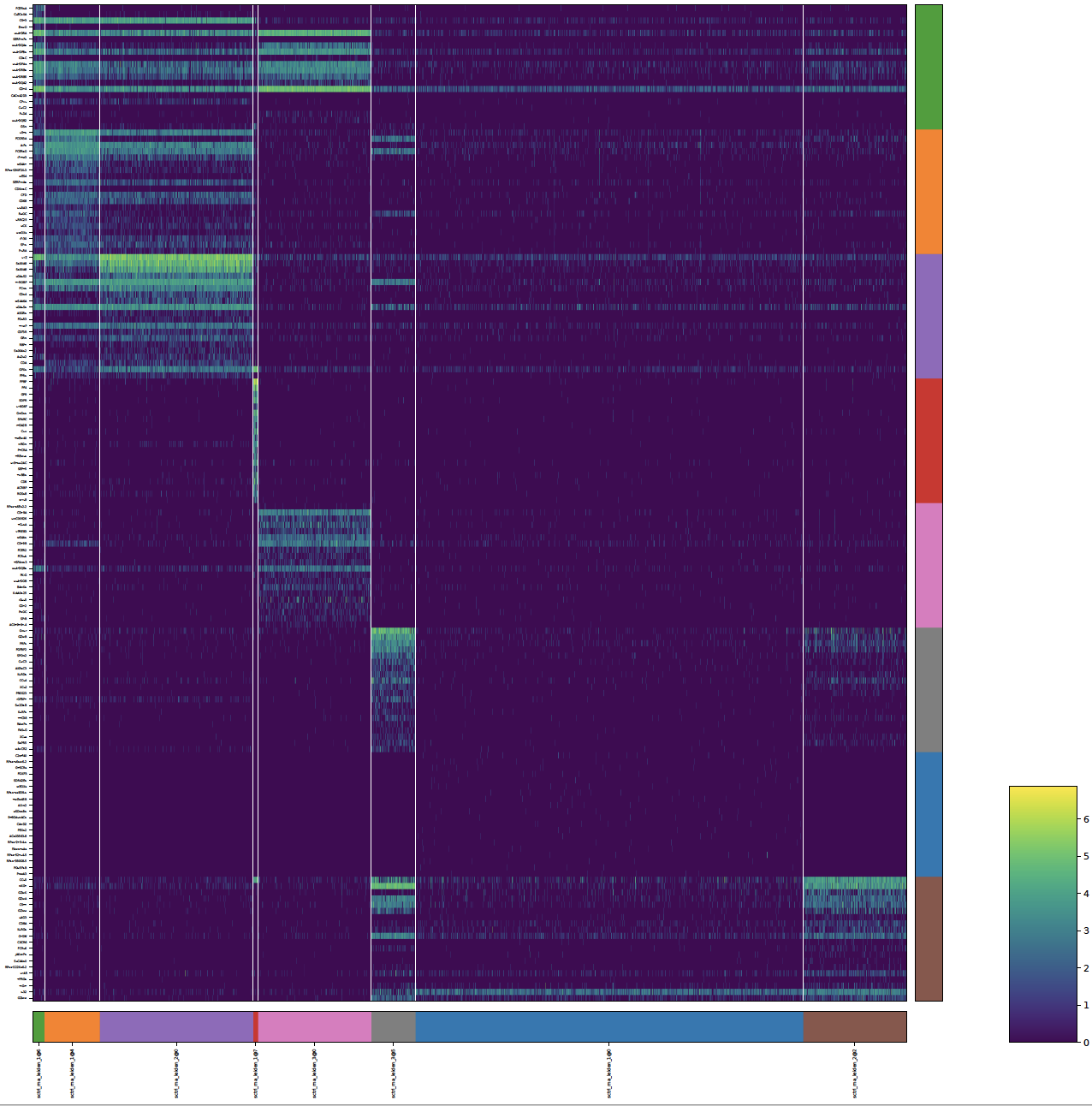
plot_long_heatmap()

sctriangulate.main_class.ScTriangulate.plot_long_heatmap(self, clusters=None, key='pruned', n_features=5, mode='marker_genes', cmap='viridis', save=True, format='pdf', figsize=(6, 4.8), feature_fontsize=3, cluster_fontsize=5, heatmap_regex=None, heatmap_direction='include')

the default scanpy heatmap is not able to support the display of arbitrary number of marker genes for each clusters, the max feature is 50. this heatmap allows you to specify as many marker genes for each cluster as possible, and the gene name will all the displayed.

Parameters

• clusters – list, what clusters we want to consider under a certain annotation.

• key – string, annotation name.

• n_features – int, the number of features to display.

• mode – string, either ‘marker_genes’ or ‘exclusive_genes’.

• cmap – string, matplotlib cmap string.

• save – boolean, whether to save or not.

• format – string, which format to save.

• figsize – tuple, the width and the height of the plot.

• feature_fontsize – int/float. the fontsize for the feature.

• cluster_fontsize – int/float, the fontsize for the cluster.

• heatmap_regex – None or a raw string for example r’^AB_’ (meaning selecing all ADT features as scTriangulate by default prefix ADT features will AB_), the usage of that is to only display certain features from certain modlaities. The underlying implementation is just a regular expression selection.

• heatmap_direction – string, ‘include’ or ‘exclude’, it is along with the heatmap_regex parameter, include means doing positive selection, exclude means to exclude the features that match with the heatmap_regex

Examples:

sctri.plot_long_umap(n_features=20,figsize=(20,20))

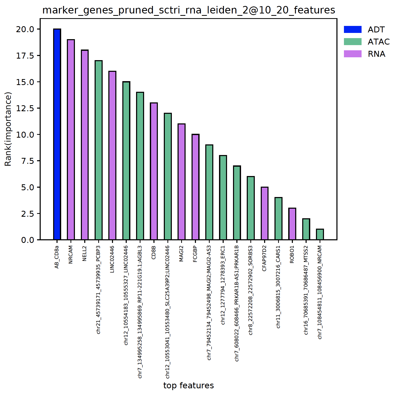
plot_multi_modal_feature_rank()

sctriangulate.main_class.ScTriangulate.plot_multi_modal_feature_rank(self, cluster, mode='marker_genes', key='pruned', tops=20, regex_dict={'adt': '^AB_', 'atac': '^chr\\d{1,2}'}, save=True, format='.pdf')

plot the top features in each clusters, the features are colored by the modality and ranked by the importance.

Parameters

• cluster – string, the name of the cluster.

• mode – string, either ‘marker_genes’ or ‘exclusive_genes’

• tops – int, top n features to plot.

• regex_adt – raw string, the pattern by which the ADT feature will be defined.

• regex_atac – raw string ,the pattern by which the atac feature will be defined.

• save – boolean, whether to save the figures.

• format – string, the format the figure will be saved.

Examples:

sctri.plot_multi_modal_feature_rank(cluster='sctri_rna_leiden_2@10')

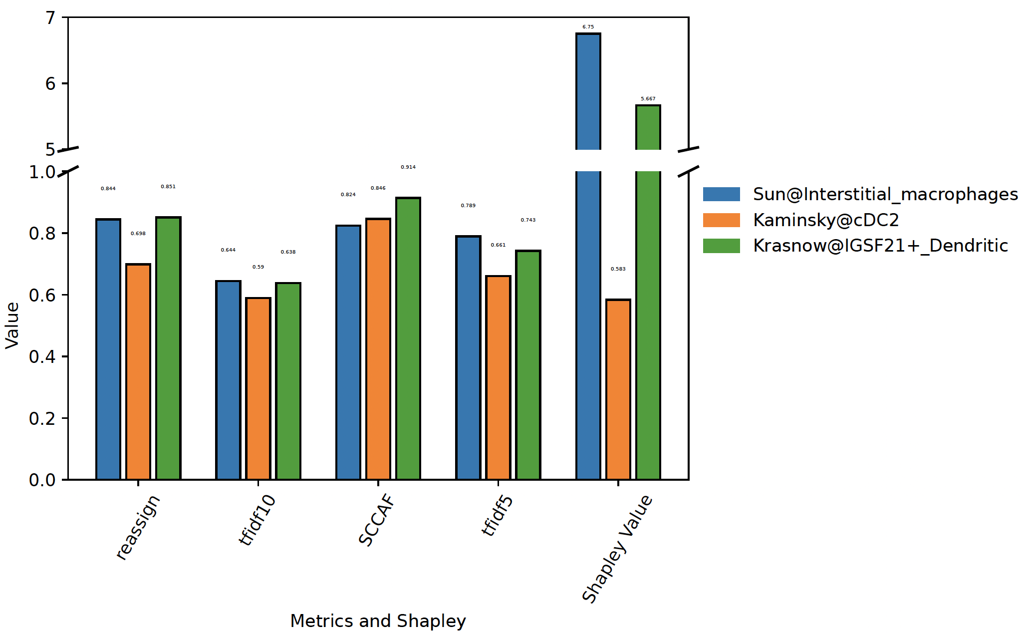
plot_stability()

sctriangulate.main_class.ScTriangulate.plot_stability(self, clusters, broke=True, height_ratios=(0.3, 0.7), hspace=0.1, text_above=0.1, top_ylim=(6, 7), bottom_ylim=(0, 1), break_point_length=0.015)

When specifying a list of clutsers, we will plot the stability metrics and shapley values associated with these clustes, This can give an intuitive view regarding which cluster is better

Parameters

• clusters – a list of clusters, each cluster should be annotation@cluster_name

• broke – bool, whether to draw barplot with break point or not, default is True

• height_ratios – tuple, the height ratios for top ax and bottom ax

• hspace – float, the space between top ax and bottom ax

• text_above – float, the distance above the bar to draw text

• top_ylim – tuple, the ylim of top ax

• bottom_ylim – tuple, the ylim of bottom ax

• break_point_length – float, to draw a tick to show break point, the length is default to 0.015

Examples:

sctri.plot_stability(clusters=['Sun@Interstitial_macrophages','Kaminsky@cDC2','Krasnow@IGSF21+_Dendritic'],broke=True,top_ylim=[5,7])
sctri.plot_stability(clusters=['Sun@monocytes','Kaminsky@cMonocyte','Kaminsky@ncMonocyte'])

plot_two_column_sankey()

sctriangulate.main_class.ScTriangulate.plot_two_column_sankey(self, left_annotation, right_annotation, opacity=0.6, pad=3, thickness=10, margin=300, text=True, save=True)

sankey plot to show the correpondance between two annotation, for example, annotation1 and annotation2, how many cells from each cluster in annotation1 will flow to each cluster in annotation2.

Parameters

• left_annotation – a string, the name of the annotation1

• right_annotation – a string, the name of the annotation2

• opacity – float number, default is 0.6, the opacity of the sankey strips

• pad – float number, default is 3, the gap between blocks vertically

• thickness – float number, default is 10, the width of each block

• margin – the white margin of the sankey plot, large value means the sankey plot will not consume the whole horizontal space (shrinkaged), default is 300

• text – whether to show the text or not, default is True, only set to False if you want to have publication quality static figure, because plotly will add a weired background shady effect on the text, not good for publication, so you can fisrt remove text, then add it back youself manually

• save – wheter to save or not, default is True.

Example:

sctri.plot_two_column_sankey('leiden1','leiden2',margin=5)

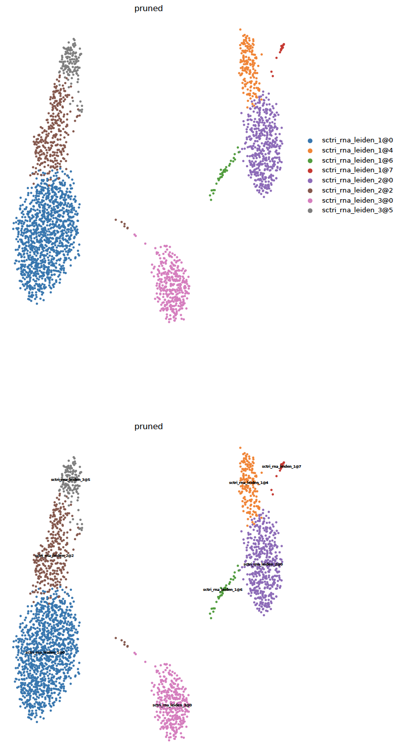
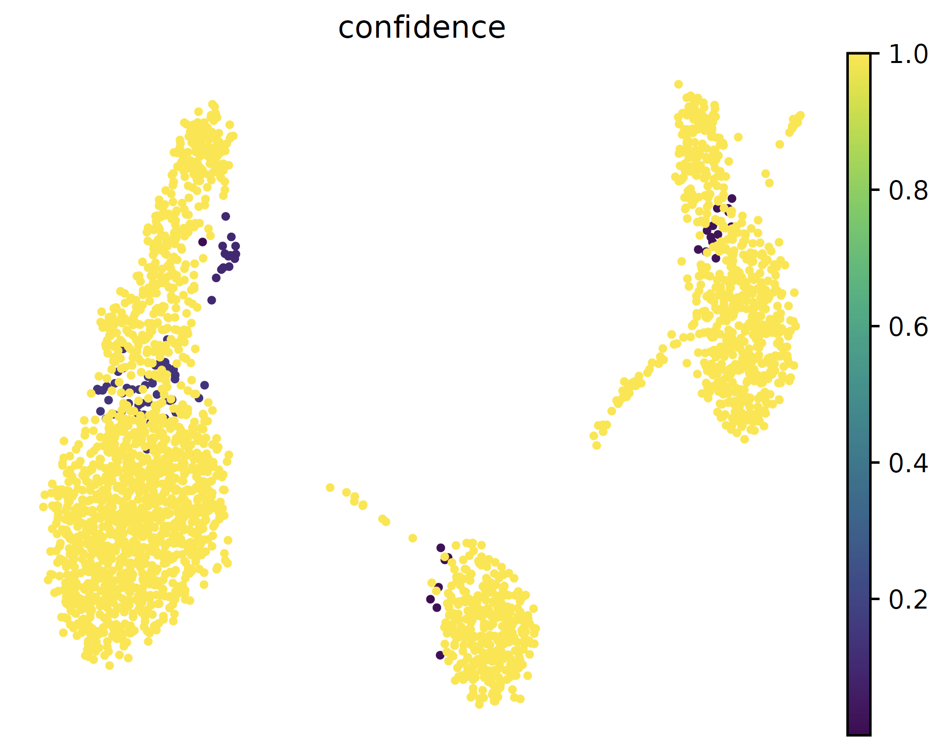
plot_umap()

sctriangulate.main_class.ScTriangulate.plot_umap(self, col, kind='category', save=True, format='pdf', umap_dot_size=None, umap_cmap='YlOrRd', frameon=False)

plotting the umap with either category cluster label or continous metrics are important. Different from the scanpy vanilla plot function, this function automatically generate two umap, one with legend on side and another with legend on data, which usually will be very helpful imagine you have > 40 clusters. Secondly, we automatically make all the background dot as light grey, instead of dark color.

Parameters

• col – string, which column in self.adata.obs that we want to plot umap from.

• kind – string, either ‘category’ or ‘continuous’

• save – boolean, whether to save it to disk or not. Default: True

• format – string. Which format to save. Default: ‘.pdf’

• umap_dot_size – int/float. the size of dot in scatter plot, if None, using scanpy formula, 120000/n_cells

• umap_cmap – string, the matplotlib colormap to use. Default: ‘YlOrRd’

• frameon – boolean, whether to have the frame on the umap. Default: False

Examples:

sctri.plot_umap(col='pruned',kind='category')
sctri.plot_umap(col='confidence',kind='continous')

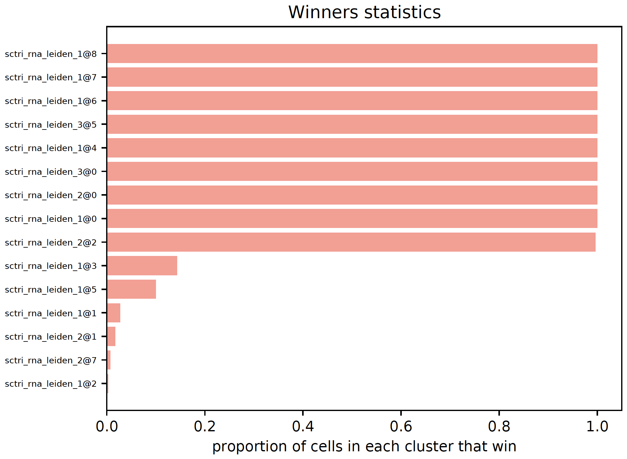
plot_winners_statistics()

sctriangulate.main_class.ScTriangulate.plot_winners_statistics(self, col, fontsize=3, plot=True, save=True)

For triangulated clusters, either ‘raw’ or ‘pruned’, visualize what fraction of cells won the game. A horizontal barplot will be generated and a dataframe with winners statistics will be returned.

Parameters

• col – string, either ‘raw’ or ‘pruned’

• fontsize – int, the fontsize for the y-label. Default: 3

• plot – boolean, whether to plot or not. Default: True

• save – boolean, whether to save the plot to the sctri.dir or not. Default: True

Returns

DataFarme

Examples:

sctri.plot_winners_statistics(col='raw',fontsize=4)

pruning()

sctriangulate.main_class.ScTriangulate.pruning(self, method='reassign', discard=None, scale_sccaf=True, layer=None, abs_thresh=10, remove1=True, reference=None, parallel=True, assess_raw=False)

Main function. After running compute_shapley, we get raw cluster results. Althought the raw cluster is informative, there maybe some weired clusters that accidentally win out which doesn’t attribute to its biological stability. For example, a cluster that only has 3 cells, or very unstable cluster. To ensure the best results, we apply a post-hoc assessment onto the raw cluster result, by applying the same set of metrics function to assess the robustness/stability of the raw clusters itself. And we will based on that to perform some pruning to get rid of unstable clusters. Finally, the cells within these clusters will be reassigned to thier nearest neighbors.

Parameters

• method – string, valid value: ‘reassign’, ‘rank’. rank will compute the metrics on all the raw clusters, together with the discard parameter which automatically discard clusters ranked at the bottom to remove unstable clusters. reassign will just remove clusters that either has less than abs_thresh cells or are in the self.invalid attribute list.

• discard – int. Least {discard} stable clusters to remove. Default: None, means just rank without removing.

• scale_sccaf – boolean. whether to scale the expression data. See compute_metrics for full explanation. Default: True

• abs_thresh – int. clusters have less than {abs_thresh} cells will be discarded in reassign mode.

• remove1 – boolean. When reassign the cells in the dicarded clutsers, whether to also reassign the cells who are the only one in each reference cluster. Default: True

• reference – string. which annotation will serve as the reference.

• parallel – boolean, whether to perform this step in parallel. (scatter and gather).Default is True

• assess_raw – boolean, whether to run the same set of cluster stability metrics on the raw cluster. Default is False

Examples:

sctri.pruning(method='pruning',discard=None)  # just assess and rank the raw clusters
sctri.pruning(method='reassign',abs_thresh=10,remove1=True,reference='annotation1')  # remove invalid clusters and reassign the cells within

regress_out_size_effect()

sctriangulate.main_class.ScTriangulate.regress_out_size_effect(self, regressor='background_zscore')

An optional step to regress out potential confounding effect of cluster_size on the metrics. Run after compute_metrics step but before compute_shapley step. All the metrics in selfadata.obs and self.score will be modified in place.

Parameters

regressor – string. which regressor to choose, valid values: ‘background_zscore’, ‘background_mean’, ‘GLM’, ‘Huber’, ‘RANSAC’, ‘TheilSen’

Example:

sctri.regress_out_size(regressor='Huber')

run_single_key_assessment()

sctriangulate.main_class.ScTriangulate.run_single_key_assessment(self, key, scale_sccaf, layer, added_metrics_kwargs)

this is a very handy function, given a set of annotation, this function allows you to assess the biogical robustness based on the metrics we define. The obtained score and cluster information will be automatically saved to self.cluster and self.score, and can be further rendered by the scTriangulate viewer.

Parameters

• key – string, the annotation/column name to assess the robustness.

• scale_sccaf – boolean, whether to scale the expression data before running SCCAF score. See compute_metrics function for full information.

• layer – see lazy_run for detail

• added_metrics_kwargs – see lazy_run for detail

Examples:

sctri.run_single_key_assessment(key='azimuth',scale_sccaf=True)

serialize()

sctriangulate.main_class.ScTriangulate.serialize(self, name='sctri_pickle.p')

serialize the sctri object through pickle protocol to the disk

Parameters

name – string, the name of the pickle file on the disk. Default: sctri_pickle.p

Examples:

sctri.serialize()

viewer_cluster_feature_figure()

sctriangulate.main_class.ScTriangulate.viewer_cluster_feature_figure(self, parallel=False, select_keys=None, other_umap=None)

Generate all the figures for setting up the viewer cluster page.

Parameters

• parallel – boolean, whether to run it in parallel, only work in some linux system, so recommend to not set to True.

• select_keys – list, what annotations’ cluster we want to inspect.

• other_umap – ndarray,replace the umap with another set.

Examples:

sctri.viewer_cluster_feature_figure(parallel=False,select_keys=['annotation1','annotation2'],other_umap=None)

viewer_cluster_feature_html()

sctriangulate.main_class.ScTriangulate.viewer_cluster_feature_html(self)

Setting up the viewer cluster page.

Examples:

sctri.viewer_cluster_feature_html()

viewer_heterogeneity_figure()

sctriangulate.main_class.ScTriangulate.viewer_heterogeneity_figure(self, key, other_umap=None, format='png', heatmap_scale=False, heatmap_cmap='viridis', heatmap_regex=None, heatmap_direction='include', heatmap_n_genes=None, heatmap_cbar_scale=None)

Generating the figures for the viewer heterogeneity page

Parameters

• key – string, which annotation to inspect the heterogeneity.

• other_umap – ndarray, replace with other umap embedding.

Examples:

sctri.viewer_heterogeneity_figure(key='annotation1',other_umap=None)

viewer_heterogeneity_html()

sctriangulate.main_class.ScTriangulate.viewer_heterogeneity_html(self, key)

Setting up viewer heterogeneity page

Parameters

key – string, which annotation to inspect.

Examples:

sctri.viewer_heterogeneity_html(key='annotation1')

Preprocessing Module

GeneConvert Class

class sctriangulate.preprocessing.GeneConvert

A collection of gene symbol conversion functions.

Now support:

1. ensemblgene id to gene symbol.

static ensemblgene_to_symbol(query, species)

Examples:

from sctriangulate.preprocessing import GeneConvert
converted_list = GeneConvert.ensemblgene_to_symbol(['ENSG00000010404','ENSG00000010505'],species='human')

Normalization Class

class sctriangulate.preprocessing.Normalization

a series of Normalization functions

Now support:

1. CLR normalization

2. total count normalization (CPTT, CPM)

3. GMM normalization

static CLR_normalization(mat)

Examples:

from sctriangulate.preprocessing import Normalization
post_mat = Normalization.CLR_normalization(pre_mat)

static GMM_normalization(mat, non_negative=False)

This method is a re-implementaion from Stephenson et al, The raw counts are first subjected to a CPTT total normalization, then a GaussianMixture model was fitted to the data, we substract the mean of the background from the data to remove background noise. Optionally, user can make the post-processed matrix as non-negative by setting non_negative==True

Examples:

from sctriangulate.preprocessing import Normalization
post_mat = Normalization.GMM_normalization(pre_mat)

static total_normalization(mat, target=10000.0)

Examples:

from sctriangulate.preprocessing import Normalization
post_mat = Normalization.total_normalization(pre_mat)

small_txt_to_adata()

sctriangulate.preprocessing.small_txt_to_adata(int_file, gene_is_index=True, sep='\t')

given a small dense expression (<2GB) txt file, load them into memory as adata, and also make sure the X is sparse matrix.

Parameters

• int_file – string, path to the input txt file, delimited by tab

• gene_is_index – boolean, whether the gene/features are the index

• sep – the delimieter, default is tab

Returns

AnnData

Exmaples:

from sctriangulate.preprocessing import small_txt_to_adata
adata= = small_txt_to_adata('./input.txt',gene_is_index=True)

large_txt_to_mtx()

sctriangulate.preprocessing.large_txt_to_mtx(int_file, out_folder, gene_is_index=True, type_convert_to='int16', n_lines=None, sep='\t')

Given a large txt dense expression file, convert them to mtx file on cluster to facilitate future I/O

Parameters

• int_file – string, path to the intput txt file, delimited by tab

• out_folder – string, path to the output folder where the mtx file will be stored

• gene_is_index – boolean, whether the gene/features is the index in the int_file.

• type_convert_to – string, since it is a large dataframe, need to read in chunk, to accelarate it and reduce the memory footprint, we convert it to either ‘int16’ if original data is count, or ‘float32’ if original data is normalized data.

• n_lines – int, the number of lines for the int_file, it is just for informative progress bar

• sep – string, defalut is tab, can be other as well

Examples:

from sctriangulate.preprocessing import large_txt_to_mtx
large_txt_to_mtx(int_file='input.txt',out_folder='./data',gene_is_index=False,type_convert_to='float32')

mtx_to_adata()

sctriangulate.preprocessing.mtx_to_adata(int_folder, gene_is_index=True, feature='genes.tsv', feature_col='index', barcode='barcodes.tsv', barcode_col='index', matrix='matrix.mtx')

convert mtx file to adata in RAM, make sure the X is sparse. Gzip file is supported as well, program will automatically detect gz extension and use gzip pacakge to read it into memory

Parameters

• int_folder – string, folder where the mtx files are stored.

• gene_is_index – boolean, whether the gene is index.

• feature – string, the name of the feature file, default for rna is genes.tsv

• feature_col – ‘index’ as index, or a int (which column, python is zero based) to use in your feature.tsv as feature

• barcode – string, the name of the barcode file, default is barcodes.tsv

• barcode_col – ‘index’ as index, or a int (which column, python is zero based) to use in your barcodes.tsv as barcode

• matrix – string, the name of the sparse matrix

Returns

AnnData

Examples:

from sctriangulate.preprocessing import mtx_to_adata
mtx_to_adata(int_folder='./data',gene_is_index=False,feature='genes')

mtx_to_large_txt()

sctriangulate.preprocessing.mtx_to_large_txt(int_folder, out_file, gene_is_index=False)

convert mtx back to large dense txt expression dataframe.

Parameters

• int_folder – string, path to the input mtx folder.

• out_file – string, path to the output txt file.

• gene_is_index – boolean, whether the gene is the index.

Examples:

from sctriangulate.preprocessing import mtx_to_large_txt
mtx_to_large_txt(int_folder='./data',out_file='input.txt',gene_is_index=False)

adata_to_mtx()

sctriangulate.preprocessing.adata_to_mtx(adata, gene_is_index=True, var_column=None, obs_column=None, outdir='data')

write a adata to mtx file

Parameters

• adata – AnnData, the adata to convert

• gene_is_index – boolean, for the resultant mtx, will gene be the index or feature is the index

• var_column – list, the var columns to write the genes.tsv, None will write all available columns

• obs_column – list, the obs columns to write the barcodes.tsv, None will write all available columns

• outdir – string, the name of the mtx folder, default is data

Example:

adata_to_mtx(adata,True,None,None,'data')

add_azimuth()

sctriangulate.preprocessing.add_azimuth(adata, result, name='predicted.celltype.l2')

a convenient function if you have azimuth predicted labels in hand, and want to add the label to the adata.

Parameters

• adata – AnnData

• result – string, the path to the ‘azimuth_predict.tsv’ file

• name – string, the column name where the user want to transfer to the adata.

Examples:

from sctriangulate.preprocessing import add_azimuth
add_azimuth(adata,result='./azimuth_predict.tsv',name='predicted.celltype.l2')

add_annotations()

sctriangulate.preprocessing.add_annotations(adata, inputs, cols_input, index_col=0, cols_output=None, sep='\t', kind='disk')

Adding annotations from external sources to the adata

Parameters

• adata – Anndata

• inputs – string, path to the txt file where the barcode to cluster label information is stored.

• cols_input – list, what columns the users want to transfer to the adata.

• index_col – int, for the input, which column will serve as the index column

• cols_output – list, corresponding to the cols_input, how these columns will be named in the adata.obs columns

• sep – string, default is tab

• kind – a string, either ‘disk’, or ‘memory’, disk means the input is the path to the text file, ‘memory’ means the input is the variable name in the RAM that represents the dataframe

Examples:

from sctriangulate.preprocessing import add_annotations
add_annotations(adata,inputs='./annotation.txt',cols_input=['col1','col2'],index_col=0,cols_output=['annotation1','annontation2'],kind='disk')
add_annotations(adata,inputs=df,cols_input=['col1','col2'],index_col=0,cols_output=['annotation1','annontation2'],kind='memory')

add_umap()

sctriangulate.preprocessing.add_umap(adata, inputs, mode, cols=None, index_col=0, key='X_umap')

if umap embedding is pre-computed, add it back to adata object.

Parameters

• adata – Anndata

• inputs – string, path to the the txt file where the umap embedding was stored.

• mode –

  string, valid value ‘pandas_disk’, ‘pandas_memory’, ‘numpy’

  • pandas_disk: the inputs argument should be the path to the txt file

  • pandas_memory: the inputs argument should be the name of the pandas dataframe in the program, inputs=df

  • numpy, the inputs argument should be a 2D ndarray contains pre-sorted (same order as barcodes in adata) umap coordinates

• cols – list, what columns contain umap embeddings

• index_col – int, which column will serve as the index column.

• key – string, the key name to add to obsm

Examples:

from sctriangulate.preprocessing import add_umap
add_umap(adata,inputs='umap.txt',mode='pandas_disk',cols=['umap1','umap2'],index_col=0)

doublet_predict()

sctriangulate.preprocessing.doublet_predict(adata)

wrapper function for running srublet, a new column named ‘doublet_scores’ will be added to the adata

Parameters

adata – Anndata

Returns

dict

Examples:

from sctriangulate.preprocessing import doublet_predict
mapping = doublet_predict(old_adata)

make_sure_adata_writable()

sctriangulate.preprocessing.make_sure_adata_writable(adata, delete=False)

maks sure the adata is able to write to disk, since h5 file is stricted typed, so no mixed dtype is allowd. this function basically is to detect the column of obs/var that are of mixed types, and delete them.

Parameters

• adata – Anndata

• delete – boolean, False will just print out what columns are mixed type, True will automatically delete those columns

Returns

Anndata

Examples:

from sctriangulate.preprocessing import make_sure_adata_writable
make_sure_adata_writable(adata,delete=True)

just_log_norm()

sctriangulate.preprocessing.just_log_norm()

perform CPTT and log operation on adata.X in place, no return value

Parameters

adata – the anndata to perform operations on

Example:

just_log_norm(adata)

scanpy_recipe()

sctriangulate.preprocessing.scanpy_recipe(adata, species='human', is_log=False, resolutions=[1, 2, 3], modality='rna', umap=True, save=True, pca_n_comps=None, n_top_genes=3000)

Main preprocessing function. Run Scanpy normal pipeline to achieve Leiden clustering with various resolutions across multiple modalities.

Parameters

• adata – Anndata

• species – string, ‘human’ or ‘mouse’

• is_log – boolean, whether the adata.X is count or normalized data.

• resolutions – list, what leiden resolutions the users want to obtain.

• modality – string, valid values: ‘rna’,’adt’,’atac’, ‘binary’[mutation data, TCR data, etc]

• umap – boolean, whether to compute umap embedding.

• save – boolean, whether to save the obtained adata object with cluster label information in it.

• pca_n_comps – int, how many PCs to keep when running PCA. Suggestion: RNA (30-50), ADT (15), ATAC (100)

• n_top_genes – int, how many features to keep when selecting highly_variable_genes. Suggestion: RNA (3000), ADT (ignored), ATAC (50000-100000)

Returns

Anndata

Examples:

from sctriangulate.preprocessing import scanpy_recipe
# rna
adata = scanpy_recipe(adata,is_log=False,resolutions=[1,2,3],modality='rna',pca_n_comps=50,n_top_genes=3000)
# adt
adata = scanpy_recipe(adata,is_log=False,resolutions=[1,2,3],modality='adt',pca_n_comps=15)
# atac
adata = scanpy_recipe(adata,is_log=False,resolutions=[1,2,3],modality='atac',pca_n_comps=100,n_top_genes=100000)
# binary
adata = scanpy_recipe(adata,resolutions=[1,2,3],modality='binary')

concat_rna_and_other()

sctriangulate.preprocessing.concat_rna_and_other(adata_rna, adata_other, umap, umap_key, name, prefix)

concatenate rna adata and another modality’s adata object

Parameters

• adata_rna – AnnData

• adata_other – Anndata

• umap – string, whose umap to use, either ‘rna’ or ‘other’

• umap_key – string, either ‘X_umap’ or ‘X_tsne’ or other string for obsm key

• name – string, the name of other modality, for example, ‘adt’ or ‘atac’

• prefix – string, the prefix added in front of features from other modality, by scTriangulate convertion, adt will be ‘AB_’, atac will be ‘’.

Return adata_combine

Anndata

Examples:

from sctriangulate.preprocessing import concat_rna_and_other
concat_rna_and_other(adata_rna,adata_adt,umap='rna',name='adt',prefix='AB_') 

nca_embedding()

sctriangulate.preprocessing.nca_embedding(adata, nca_n_components, label, method, max_iter=50, plot=True, save=True, format='pdf', legend_loc='on data', n_top_genes=None, hv_features=None, add_features=None)

Doing Neighborhood component ananlysis (NCA), so it is a supervised PCA that takes the label from the annotation, and try to generate a UMAP embedding that perfectly separate the labelled clusters.

Parameters

• adata – the Anndata

• nca_n_components – recommend to be 10 based on Ref

• label – string, the column name which contains the label information

• method – either ‘umap’ or ‘tsne’

• max_iter – for the NCA, default is 50, it is generally good enough

• plot – whether to plot the umap/tsne or not

• save – whether to save the plot or not

• format – the saved format, default is ‘pdf’

• legend_loc – ‘on data’ or ‘right margin’

• n_top_genes – how many hypervariable genes to choose for NCA, recommended 3000 or 5000, default is None, means there will be other features to add, multimodal setting

• hv_features – a list contains the user-supplied hypervariable genes/features, in multimodal setting, this can be [rna genes] + [ADT protein]

• add_features – this should be another adata contains features from other modalities, or None means just for RNA

Example:

from sctriangulate.preprocessing import nca_embedding
# only RNA
nca_embedding(adata,nca_n_components=10,label='annotation1',method='umap',n_top_genes=3000)
# RNA + ADT
# list1 contains [gene features that are variable] and [ADT features that are variable]
nca_embedding(adata_rna,nca_n_components=10,label='annotation1',method='umap',n_top_genes=3000,hv_features=list1, add_features=adata_adt)

umap_dual_view_save()

sctriangulate.preprocessing.umap_dual_view_save(adata, cols, method='umap')

generate a pdf file with two umap up and down, one is with legend on side, another is with legend on data. More importantly, this allows you to generate multiple columns iteratively.

Parameters

• adata – Anndata

• cols – list, all columns from which we want to draw umap.

• method – string, either umap or tsne

Examples:

from sctriangulate.preprocessing import umap_dual_view_save
umap_dual_view_save(adata,cols=['annotation1','annotation2','total_counts'])

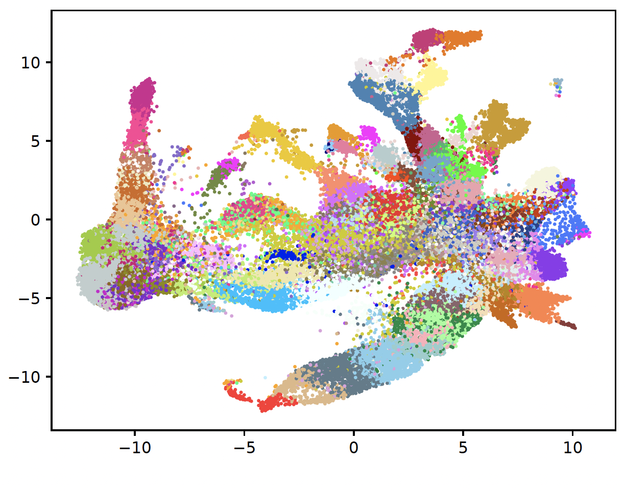
umap_color_exceed_102()

sctriangulate.preprocessing.umap_color_exceed_102(adata, key, dot_size=None, legend_fontsize=6, outdir='.', name=None, **kwargs)

draw a umap that bypass the scanpy 102 color upper bound, this can generate as many as 433 clusters.

Parameters

• adata – Anndata

• key – the categorical column in adata.obs, which will be plotted

• dot_size – None or number

• legend_fontsize – defualt is 6

• outdir – output directory, default is ‘.’

• name – name of the plot, default is None

Exmaple:

from sctriangulate.preprocessing import umap_color_exceed_102
umap_color_exceed_102(adata,key='leiden6')  # more than 130 clusters

make_sure_mat_dense()

sctriangulate.preprocessing.make_sure_mat_dense(mat)

make sure a matrix is dense

Parameters

mat – ndarary

Return mat

ndarray (dense)

Examples:

mat = make_sure_mat_dense(mat)

make_sure_mat_sparse()

sctriangulate.preprocessing.make_sure_mat_sparse(mat)

make sure a matrix is sparse

Parameters

mat – ndarary

Return mat

ndarray (sparse)

Examples:

mat = make_sure_mat_dense(mat)

gene_activity_count_matrix_old_10x()

sctriangulate.preprocessing.gene_activity_count_matrix_old_10x(fall_in_promoter, fall_in_gene, valid=None)

this function is to generate gene activity count matrix, please refer to gene_activity_count_matrix_new_10x for latest version of 10x fragements.tsv output.

how to get these two arguments? (LIGER team approach)

1. sort the fragment, gene and promoter bed, or use function in this module to sort the reference bed files:

   sort -k1,1 -k2,2n -k3,3n pbmc_granulocyte_sorted_10k_atac_fragments.tsv > atac_fragments.sort.bed
   sort -k 1,1 -k2,2n -k3,3n hg19_genes.bed > hg19_genes.sort.bed
   sort -k 1,1 -k2,2n -k3,3n hg19_promoters.bed > hg19_promoters.sort.bed
   

2. bedmap:

   module load bedops
   bedmap --ec --delim "   " --echo --echo-map-id hg19_promoters.sort.bed atac_fragments.sort.bed > atac_promoters_bc.bed
   bedmap --ec --delim "   " --echo --echo-map-id hg19_genes.sort.bed atac_fragments.sort.bed > atac_genes_bc.bed
   

the following was taken from http://htmlpreview.github.io/?https://github.com/welch-lab/liger/blob/master/vignettes/Integrating_scRNA_and_scATAC_data.html

• delim. This changes output delimiter from ‘|’ to indicated delimiter between columns, which in our case is “ ”.

• ec. Adding this will check all problematic input files.

• echo. Adding this will print each line from reference file in output. The reference file in our case is gene or promoter index.

• echo-map-id. Adding this will list IDs of all overlapping elements from mapping files, which in our case are cell barcodes from fragment files.

3. Finally:

   from sctriangulate.preprocessing import gene_activity_count_matrix_old_10x
   gene_activity_count_matrix_old_10x(fall_in_promoter,fall_in_gene,valid=None)
   

gene_activity_count_matrix_new_10x()

sctriangulate.preprocessing.gene_activity_count_matrix_new_10x(fall_in_promoter, fall_in_gene, valid=None)

Full explanation please refer to gene_activity_count_matrix_old_10x

Examples:

from sctriangulate.preprocessing import gene_activity_count_matrix_new_10x
gene_activity_count_matrix_new_10x(fall_in_promoter,fall_in_gene,valid=None)       

format_find_concat()

sctriangulate.preprocessing.format_find_concat(adata, canonical_chr_only=True, gtf_file='gencode.v38.annotation.gtf', key_added='gene_annotation', **kwargs)

this is a wrapper function to add nearest genes to your ATAC peaks or bins. For instance, if the peak is chr1:55555-55566, it will be annotated as chr1:55555-55566_gene1;gene2 :param adata: The anndata, the var_names is the peak/bin, please make sure the format is like chr1:55555-55566 :param canonical_chr_only: boolean, default to True, means only contain features on canonical chromosomes. for human, it is chr1-22 and X,Y :param gtf_file: the path to the gtf files, we provide the hg38 on this google drive link to download :param key_added: string, the column name where the gene annotation will be inserted to adata.var, default is ‘gene_annotation’ :return adata: Anndata, the gene annotation will be added to var, and the var_name will be suffixed with gene annotation, if canonical_chr_only is True, then only features on canonical

chromsome will be retained.

Example::

adata = format_find_concat(adata)

find_genes()

sctriangulate.preprocessing.find_genes(adata, gtf_file, key_added='gene_annotation', upstream=2000, downstream=0, feature_type='gene', annotation='HAVANA', raw=False)

This function is taken from episcanpy. all the credits to the original developer

merge values of peaks/windows/features overlapping genebodies + 2kb upstream. It is possible to extend the search for closest gene to a given number of bases downstream as well. There is commonly 2 set of annotations in a gtf file(HAVANA, ENSEMBL). By default, the function will search annotation from HAVANA but other annotation label/source can be specifed. It is possible to use other type of features than genes present in a gtf file such as transcripts or CDS.

Examples:

from sctriangulate.preprocessing import find_genes
find_genes(adata,gtf_file='gencode.v38.annotation.gtf)

reformat_peak()

sctriangulate.preprocessing.reformat_peak(adata, canonical_chr_only=True)

To use find_genes function, please first reformat the peak from 10X format “chr1:10109-10357” to find_gene format “chr1_10109_10357”

Parameters

• adata – AnnData

• canonical_chr_only – boolean, only kept the canonical chromosome

Returns

AnnData

Examples:

from sctriangulate.preprocessing import reformat_peak
adata = reformat_peak(adata,canonical_chr_only=True)

rna_umap_transform()

sctriangulate.preprocessing.rna_umap_transform(outdir, ref_exp, ref_group, q_exp_list, q_group_list, q_identifier_list, pca_n_components, umap_min_dist=0.5)

Take a reference expression matrix (pandas dataframe), and a list of query expression matrics (pandas dataframe), along with a list of query expression identifiers. This function will generate the umap transformation of your reference exp, and make sure to squeeze your each query exp to the same umap transformation.

Parameters

• outdir – the path in which all the results will go

• ref_exp – the pandas dataframe object,index is the features, column is the cell barcodes

• ref_group – the pandas series object, index is the cell barcodes, the value is the clusterlabel information

• q_exp_list – the list of pandas dataframe object, requirement is the same as ref_exp

• q_group_list – the list of pandas series object, requirement is the same as ref_group

• q_identifier_list – the list of string, to denote the name of each query dataset

• pca_n_components – the int, denote the PCs to use for PCA

• umap_min_dist – the float number, denote the min_dist parameter for umap program

Examples:

rna_umap_transform(outdir='.',ref_exp=ref_df,ref_group=ref_group_df,q_exp_list=[q1_df],q_group_list=[q1_group_df],q_identifier_list=['q1'],pca_n_components=50)

Colors Module

color_stdout()

sctriangulate.colors.color_stdout(skk, c)

color your output to the terminal :param skk: the string you want to color :param c: the name of the color ‘red’,’green’,’yellow’,’lightpurple’,’cyan’,’lightgrey’,’black’

Example:

from color import color_stdout
# when print to terminal, it will be red
print(color_stdout('hello','red'))

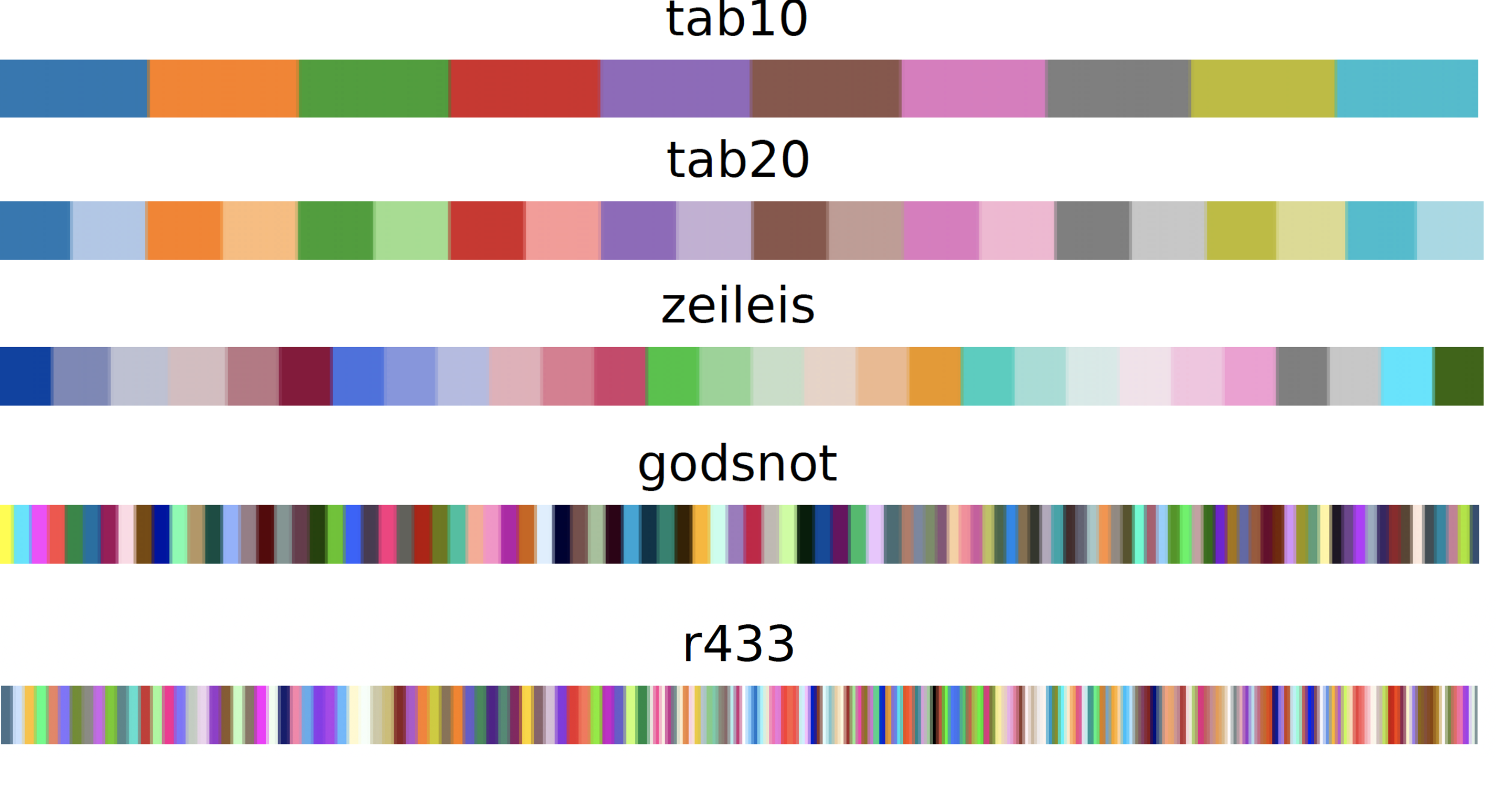
pick_n_colors()

sctriangulate.colors.pick_n_colors(n, gradient=False, cmap=None)

a very handy and abstract function, pick n colors in hex code that guarantee decent contrast.

1. n <=10, use tab10

2. 10 < n <= 20, use tab20

3. 20 < n <= 28, use zeileis (take from scanpy)

4. 28 < n <= 102, use godsnot (take from scanpy)

5. n > 102, use jet cmap (no guarantee for obvious contrast)

Parameters

• n – int, how many colors are needed

• gradient – boolean, whether to use gradient color, default is False

• cmap – string, the valid cmap to use if gradient=True

Returns

list, each item is a hex code.

Examples:

generate_block(color_list = pick_n_colors(10),name='tab10')
generate_block(color_list = pick_n_colors(20),name='tab20')
generate_block(color_list = pick_n_colors(28),name='zeileis')
generate_block(color_list = pick_n_colors(102),name='godsnot')
generate_block(color_list = pick_n_colors(200),name='433')

colors_for_set()

sctriangulate.colors.colors_for_set(setlist, **kwargs)

given a set of items, based on how many unique item it has, pick the n color

Parameters

• setlist – list without redundant items.

• **kwargs –

  will be passed to pick_n_colors function

Returns

dictionary, {each item: hex code}

Exmaples:

cmap_dict = colors_for_set(['batch1','batch2])
# {'batch1': '#1f77b4', 'batch2': '#ff7f0e'}

gradienting()

sctriangulate.colors.gradienting(input_hex, n)

Given a hex color code (pivot color), it returns a gradient (specified by n) determined by this pivot color

Parameters

• input_hex – string, like ‘#4c4cff’

• n – int, how many gradient you want

Return gradiented_hex

list, like [‘#d2d2ff’, ‘#a5a5ff’, ‘#7878ff’, ‘#4c4cff’]

Examples:

gradiented_hex = gradienting('#4c4cff',n=4)
# ['#d2d2ff', '#a5a5ff', '#7878ff', '#4c4cff']

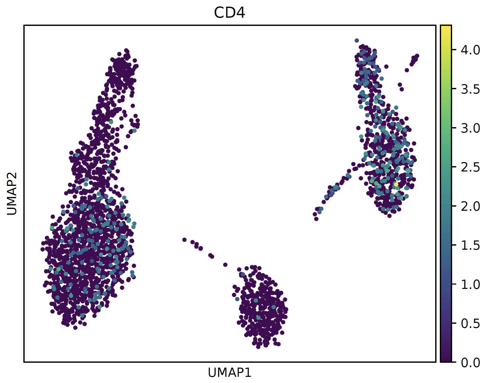
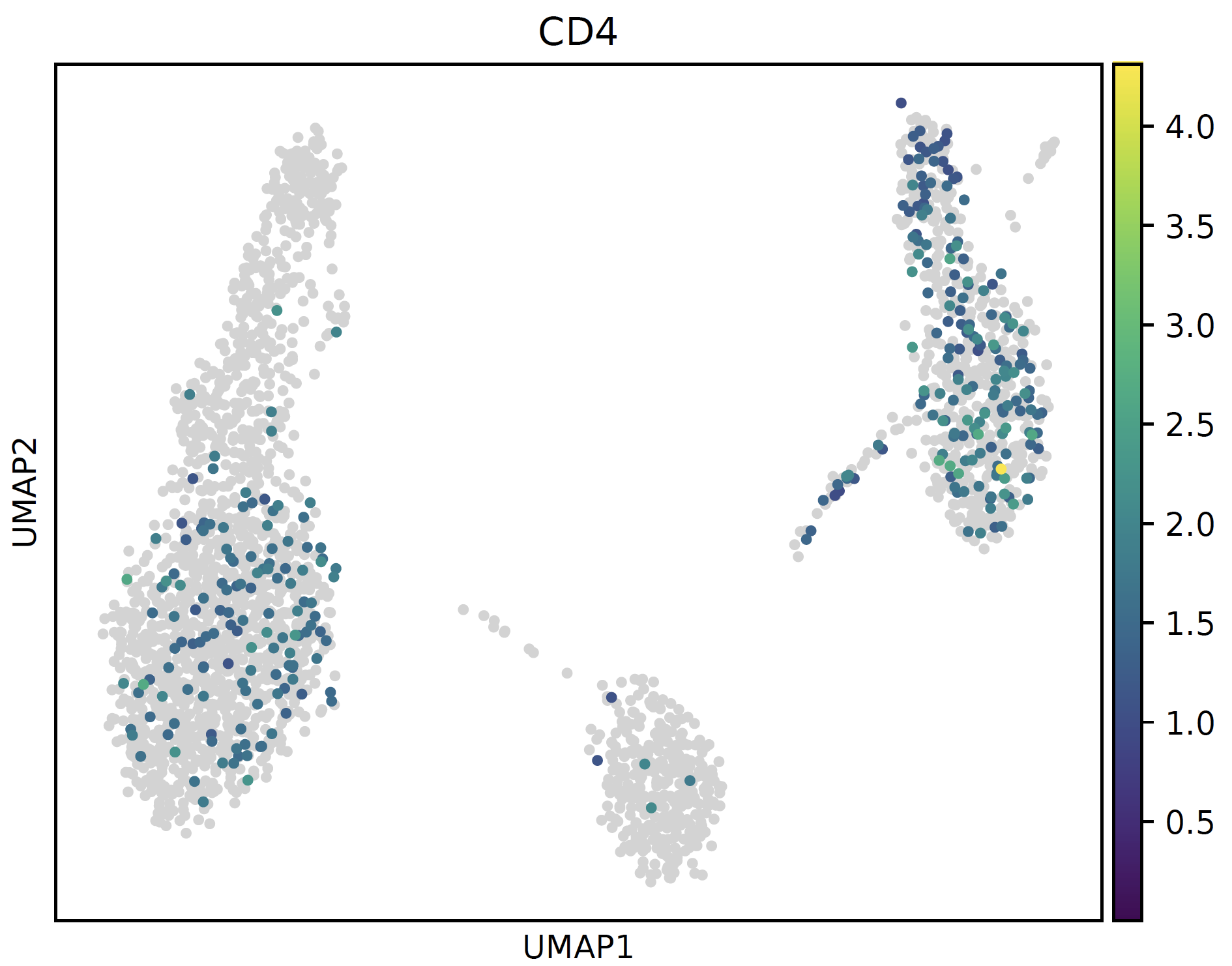
bg_greyed_cmap()

sctriangulate.colors.bg_greyed_cmap(cmap_str)

set 0 value as lightgrey, which will render better effect on umap

Parameters

cmap_str – string, any valid matplotlib colormap string

Returns

colormap object

Examples:

# normal cmap
sc.pl.umap(sctri.adata,color='CD4',cmap='viridis')
plt.savefig('normal.pdf',bbox_inches='tight')
plt.close()

# bg_greyed cmap
sc.pl.umap(sctri.adata,color='CD4',cmap=bg_greyed_cmap('viridis'),vmin=1e-5)
plt.savefig('bg_greyed.pdf',bbox_inches='tight')
plt.close()

build_custom_continuous_cmap()

sctriangulate.colors.build_custom_continuous_cmap(*rgb_list)

Generating any custom continuous colormap, user should supply a list of (R,G,B) color taking the value from [0,255], because this is the format the adobe color will output for you.

Examples:

test_cmap = build_custom_continuous_cmap([64,57,144],[112,198,162],[230,241,146],[253,219,127],[244,109,69],[169,23,69])
fig,ax = plt.subplots()
fig.colorbar(cm.ScalarMappable(norm=colors.Normalize(),cmap=diverge_cmap),ax=ax)

build_custom_divergent_cmap()

sctriangulate.colors.build_custom_divergent_cmap(hex_left, hex_right)

User supplies two arbitrary hex code for the vmin and vmax color values, then it will build a divergent cmap centers at pure white.

Examples:

diverge_cmap = build_custom_divergent_cmap('#21EBDB','#F0AA5F')
fig,ax = plt.subplots()
fig.colorbar(cm.ScalarMappable(norm=colors.Normalize(),cmap=diverge_cmap),ax=ax)

retrieve_pretty_cmap()

sctriangulate.colors.retrieve_pretty_cmap(name)

retrieve pretty customized colormap

Parameters

name – string, valid value ‘altanalyze’, ‘shap’, ‘scphere’

Returns

cmap object

Examples:

generate_gradient(cmap=retrieve_pretty_cmap('shap'),name='shap')
generate_gradient(cmap=retrieve_pretty_cmap('altanalyze'),name='altanalyze')
generate_gradient(cmap=retrieve_pretty_cmap('scphere'),name='scphere')

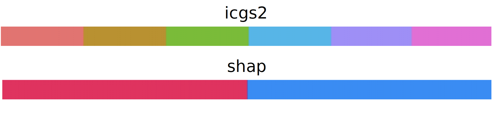
retrieve_pretty_colors()

sctriangulate.colors.retrieve_pretty_colors(name)

retrieve pretty customized colors (discrete)

Parameters

name – string, valid value ‘icgs2’, ‘shap’

Returns

list, each item is hex code

Examples:

generate_block(color_list = retrieve_pretty_colors('icgs2'),name='icgs2')
generate_block(color_list = retrieve_pretty_colors('shap'),name='shap')

generate_block()

sctriangulate.colors.generate_block(color_list, name)

Given a list of color (each item is a hex code), visualize them side by side. See example.

generate_gradient()

sctriangulate.colors.generate_gradient(cmap, name)

Given a continuous cmap, visualize them. See example.

Spatial (Experimental)

read_spatial_data

sctriangulate.spatial.read_spatial_data(mode_count='mtx', mode_spatial='visium', mtx_folder=None, txt_file=None, txt_file_sep=',', tmp_mtx_folder=None, spatial_library_id=None, spatial_folder=None, spatial_coord=None, spatial_coord_sep=',', coord_columns=None, spatial_images=None, spatial_scalefactors=None, **kwargs)

read the spatial data into the memory as adata

Parameters

• mode_count –

  string, how the spatial count data is present:

  • mtx: a folder where inputs are represented in mtx format

  • large_txt: a large txt file, usually means exceed 2GB

  • small_txt: a small txt file, usually means below 2GB

• mode_spatial –

  string, how the spatial images and associated files are present

  • visium: spatial location and images are laid out as visium format from spaceranger

  • generic: more generic format where the users have to supply the file path to find the location and images

Depending on how the mode_count is set, additional paramters need to be set for reading the count data

Parameters

• mtx_folder – string, if mode_count == ‘mtx’, specify the folder name

• txt_file_sep – string, if mode_count == ‘small_txt’ for ‘large_txt’, it can be either common or tab or others

• txt_file – string, if mode_count == ‘small_txt’ for ‘large_txt’, specify the txt path

• tmp_mtx_folder – string, if mode_count == ‘large_txt’, specify the folder where the intermediate mtx folder will be created

Depending on how the mode_spatial is set, addtiional parameters need to be set for reading the spatial data

Parameters

• spatial_library_id – string, when necessary, specify the library_id for the spatial slide

• spatial_folder – string, if mode_spatial == ‘visium’, specifiy the folder name, when mode_spatial==’visium’

• spatial_coord – string, the path to which we have spatial coords for each barcode, when mode_spatial==’generic’

• spatial_coord_sep – string, it can be ‘ ‘ or ‘,’ or other delimiters, when mode_spatial==’generic’

• coord_columns – list, the columns you need to transfer from spatial_coord, when mode_spatial ==’generic’

• spatial_images – dict, {‘hires’:path_to_image}, it can be None, when mode_spatial ==’generic’

• spatial_scalefactors – dict, {‘tissue_hires_scalef’:0.17,’tissue_lowres_scalef’:0.05,’fiducial_diameter_fullres’:144,’spot_diameter_fullres’:89}, it can be None, when mode_spatial==’generic’

Depending on how the mode_count is set, additional parameters can be passed to the underlying preprocessing functions to read in the data

Parameters

kwargs – optional keyword arguments will be passed to the function handling how the input count will be read

Examples:

id_ = '1160920F'
adata_spatial = read_spatial_data(mtx_folder='filtered_count_matrices/{}_filtered_count_matrix'.format(id_),
                                  spatial_folder='filtered_count_matrices/{}_filtered_count_matrix/{}_spatial'.format(id_,id_),
                                  spatial_library_id=id_,feature='features.tsv')

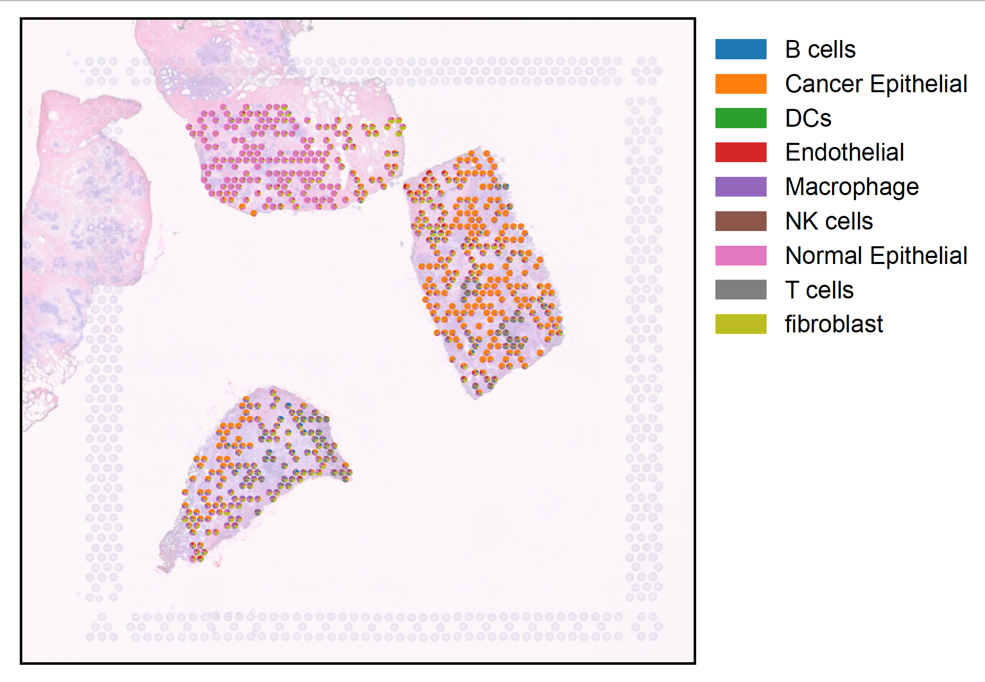
plot_deconvolution

sctriangulate.spatial.plot_deconvolution(adata, decon, fraction=0.1, size=0.5, library_id=None, alpha=0.5, outdir='.')

Visualize the deconvolution result as pie chart, serving as a complement function on top of scanpy.pl.spatial where each dot now is a pie chart

Parameters

• adata – AnnData, requires img, scale_factor, spot_diameter in the canonical slot based on squidpy convention, you can get it either using squidpy.read_visium or sctriangulate.spatial.read_spatial_data

• decon – A dataframe whose index is spot barcode, column is the cell types, value represents cell type proportion (each row sums to 1)

• fraction – float, plot that fraction of spot on the image, default is 0.1

• size – float, default is 0.5, adjust it based on visual effect

• library_id – None or string, if None, automatically extract from adata.uns[‘spatial’], or particularly specify

• alpha – float, default is 0.5, the transparency of the underlying image

• outdir – string, the output dir for saved image

Example:

decon = pd.read_csv('inputs/decon_results_A/cell2location_prop_processed.txt',index_col=0,sep=' ')
plot_deconvolution(adata_spatial,decon,fraction=0.5,alpha=0.3)

cluster_level_spatial_stability

sctriangulate.spatial.cluster_level_spatial_stability(adata, key, method, neighbor_key='spatial_distances', sparse=True, coord_type='generic', n_neighs=6, radius=None, delaunay=False)

derive optional stability score in the context of spatial transcriptomics

Parameters

• adata – the Anndata

• key – string, the column in obs to derive cluster-level stability score

• method –

  string, which score, support tbe following:

  • degree_centrality

  • closeness_centrality

  • average_clustering

  • spread

  • assortativity

  • number_connected_components

• neighbor_key – string, which obsm key to use for neighbor adjancency, default is spatial_distances

• sparse – boolean, whether the adjancency matrix is sparse or not, default is True

• coord_type – string, default is generic, passed to sq.gr.spatial_neighbors()

• n_neighs – int, default is 6, passed to sq.gr.spatial_neighbors()

• radius – float or None (default), passed to sq.gr.spatial_neighbors()

• delaunay – boolean, default is False, whether to use delaunay for spatial graph, passed to sq.gr.spatial_neighbors()

Examples:

cluster_level_spatial_stability(adata,'cluster',method='centrality')
cluster_level_spatial_stability(adata,'cluster',method='spread')
cluster_level_spatial_stability(adata,'cluster',method='assortativity',neighbor_key='spatial_distances',sparse=True)
cluster_level_spatial_stability(adata,'cluster',method='number_connected_components',neighbor_key='spatial_distances',sparse=True)

create_spatial_features

sctriangulate.spatial.create_spatial_features(adata, mode, coord_type='generic', n_neighs=6, n_rings=1, radius=None, delaunay=False, sparse=True, library_id=None, img_key='hires', sf_key='tissue_hires_scalef', sd_key='spot_diameter_fullres', feature_types=['summary', 'texture', 'histogram'], feature_added_kwargs=[{}, {}, {}], segmentation_feature=False, segmentation_method='watershed')

Extract spatial features (including spatial coordinates, spatial neighbor graph, spatial image)

Parameters

• adata – the adata to extract features from

• mode –

  string, support:

  • coordinate: feature derived from pure spatial coordinates

  • graph_importance: feature derived from the spatial neighbor graph

  • tissue_images: feature derived from assciated tissue images (H&E, fluorescent)

• coord_type – string, default is generic, passed to sq.gr.spatial_neighbors()

• n_neighs – int, default is 6, passed to sq.gr.spatial_neighbors()

• n_rings – int, default is 1, passed to sq.gr.spatial_neighbors()

• radius – float or None (default), passed to sq.gr.spatial_neighbors()

• delaunay – boolean, default is False, whether to use delaunay for spatial graph, passed to sq.gr.spatial_neighbors()

• library_id – string or None, when choosing tissue_images, need to retrieve the image from adata.uns

• img_key – string, when choosing tissue_images, need to retrieve the image from adata.uns

• sf_key – string, when choosing tissue_images, we need to associate image pixel to the spot location, which relies on scalefactor

• sd_key – the string, the key of spot_diameter_fullres in adata.uns[‘spatial’][libarary_id][‘scalefactorf’]

• feature_types – list, default including summary, texture and histogram

• feature_added_kwargs – nested list, each element is a dict, containing additional keyword arguments being passed to each feature function in feature_types

• segmentation_feature – boolean, whether to extract segmentation feature or not, default is False

• segmentation_method – string the segmentation method to use, default is ‘watershed’

Examples:

# derive feature
spatial_adata_image = create_spatial_features(adata_spatial,mode='tissue_image',library_id='CID44971',img_key='hires',segmentation_feature=True)  
# derive spatial clusters
sc.pp.neighbors(spatial_adata_image)
sc.tl.leiden(spatial_adata_image)
spatial_adata_image.uns['spatial'] = adata_spatial.uns['spatial']
spatial_adata_image.obsm['spatial'] = adata_spatial.obsm['spatial']
sc.pl.spatial(spatial_adata_image,color='leiden')

identify_ecosystem

sctriangulate.spatial.identify_ecosystem(adata_spatial, coord_type='grid', n_neighbors=6, n_rings=1, include_self=True, resolution=1, save=True, outdir='.', legend_loc='right margin')

Ecosystem means the frequent interaction within one cell type, or across multiple cell types. Examples include:

1. A ecosytem within which macrophage interact with macrophage

2. A ecosytem where stroma cells encapsulating tumor tissue

3. A ecosytem where T cell and B cell co-occur

This function is inspired by the recurrent cellular neighborhood analysis described in The Spatial Landscape of Progression and Immunoediting in Primary Melanoma at Single-Cell Resolution.

Parameters

• adata_spatial – Anndata, follow the squidpy convention in terms of the slot where img, scale_factor should go into, further more, please put decon dataframe into adata_spatial.obsm[‘decon’]

• coord_type – either grid or generic, passed to sq.gr.spatial_neighbors function

• n_neighbors – int, default is 6, passed to sq.gr.spatial_neighbors function

• n_rings – int, default is 1, passed to sq.gr.spatial_neighbors function

• include_self – boolean, when counting neighbors, whether or not including the spot itself

• resolution – float, default is 1, this will be passed to leiden algorithm

• save – boolean, whether to save the plot or not

• outdir – string, default is ‘.’, output directory

• legend_loc – string, passed to sq.pl.spatial, default is right margin

Example:

adata_spatial.obsm['decon'] = decon.loc[adata_spatial.obs_names,:]
adata_neigh = identify_ecosystem(adata_spatial,n_rings=2)
sc.pl.spatial(adata_neigh,color='leiden',groups=['6'],alpha_img=0.2)

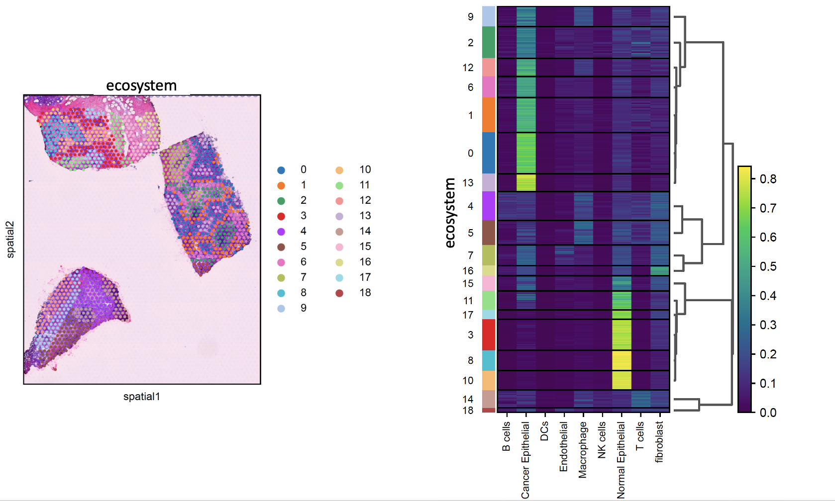
identity_spatial_program

sctriangulate.spatial.identify_spatial_program(adata_spatial, coord_type='grid', n_neighbors=6, n_rings=1, spatial_community_resolution=8, spatial_community_min_cells=10, plot=True, outdir='.', mode='spot_cell_type_proportion', n_program=10)

The most important analysis is to define spatial program, meaning spatial region that are proximal and somehow transcriptomically similar. This function provide a very flexible way to define spatial program by first derive spatial community solely based on spatial coordinates, then we merge spatial community into spatial cluster/structure such that spatial communities sharing similar gene expression or cell phenotype profile will be clustered tegether, the resultant spatial cluster represents the biologically meaningful multicellular spatial structure, it is inspired by Figure 4 in this paper.

Parameters

• adata_spatial – the Anndata with spatial coordinate

• coord_type – either grid or generic, passed to sq.gr.spatial_neighbors function

• n_neighbors – int, default is 6, passed to sq.gr.spatial_neighbors function

• n_rings – int, default is 1, passed to sq.gr.spatial_neighbors function

• spatial_community_resolution – float, default is 8, passed to nx.algorithms.community.greedy_modularity_communities, high value means smaller clusters

• spatial_community_min_cells – int, the minimum number of cells/spots that a spatial community needs to have

• plot – boolean, whether to plot spatial community and spatial cluster

• outdir – string, the path to the output dir

• mode – string, which transcriptomical profile to consider, it can be ‘spot_cell_type_proportion’ coming out of spatial deconvolution methods or spot gene expression

• n_program – int, the number of spatial program you want, it is passed to hierarchical clustering algorithm

Return df_subgragh

dataFrame, readily input for Broad Morpheus online heatmap generation tool.

Examples:

adata_spatial.obsm['decon'] = decon.loc[adata_spatial.obs_names,:]
df_subgraph = identify_spatial_program(adata_spatial,n_rings=1)