Tutorial
Single-Modality (scRNA-Seq) workflow
In this example, we are going to analyze the pbmc10k scRNA dataset downloaded from 10x official website (chemistry v3.1). This dataset has also been used as the demo query data in Azimuth. It contains 11,769 single cells before filtering.
Note
Please makse sure you have internet connection while running the tutorials, currently the program conduct gene enrichment annalysis which requires internet connection, we may remove this feature in the future.
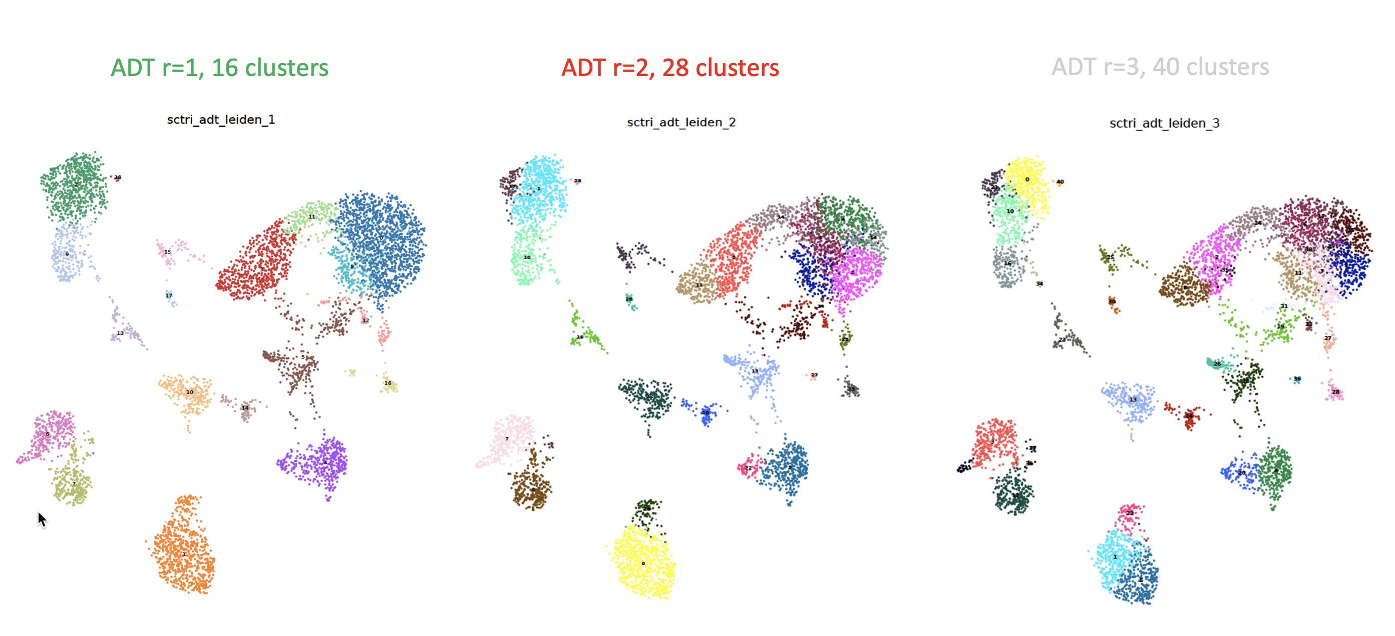
Here we first conduct basic single cell analysis to obtain Leiden clustering results, however, at various resolutions (r=1,2,3). Smaller resolutions lead to broader clusters, and larger resolution value will result in more granular clustering. We leverage scTriangulate to take the three resolutions as the query annotation-sets, and automatically mix-and-match cluster boundary from different resolutions, which at the end, yield scTriangulate reconciled cluster solutions.
Download and preprocessing
First load the packages:
import os
import sys
import scanpy as sc
from sctriangulate import *
from sctriangulate.preprocessing import *
Warning
If you experience difficulties downloading the files through the link we provided in this page, you can try to paste the link to the browser, and then add “http://” as prefix (not https) to the URL, the download will start.
The h5 file can be downloaded from http://altanalyze.org/scTriangulate/scRNASeq/pbmc_10k_v3.h5. First use the scanpy and scTriangulate preprocessing module to conduct basic quality control (QC) filtering and to run the single cell analysis pipeline:
adata = sc.read_10x_h5('./pbmc_10k_v3_filtered_feature_bc_matrix.h5')
adata.var_names_make_unique()
adata.var['mt'] = adata.var_names.str.startswith('MT-')  # annotate mitochondrial genes as 'mt'
sc.pp.calculate_qc_metrics(adata, qc_vars=['mt'], percent_top=None, log1p=False, inplace=True)
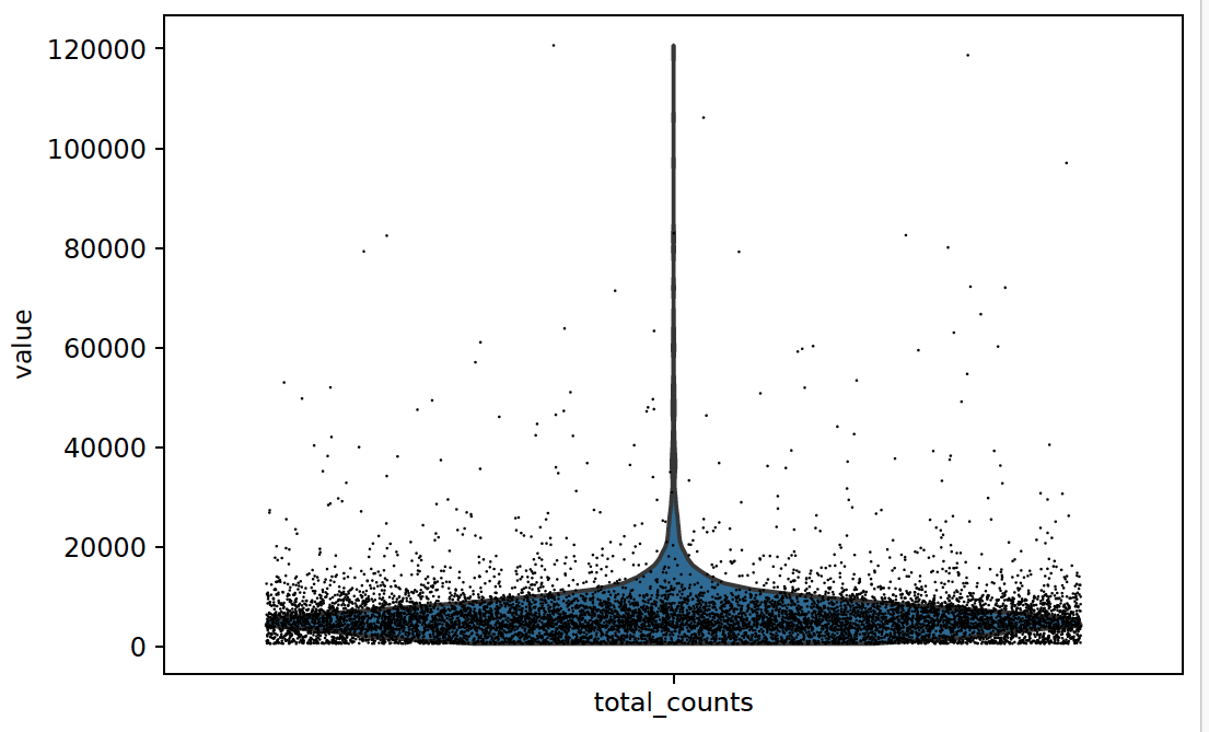
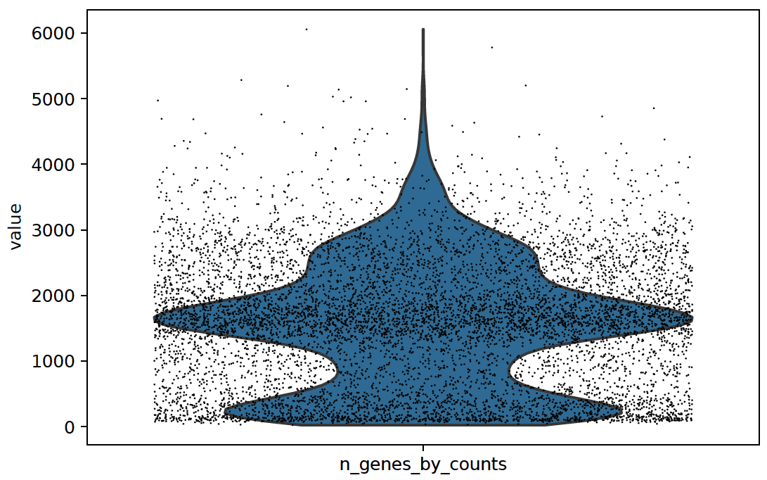
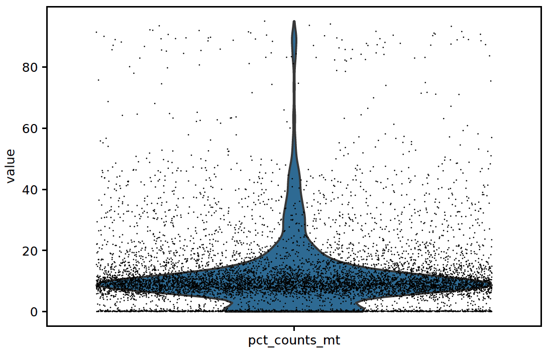
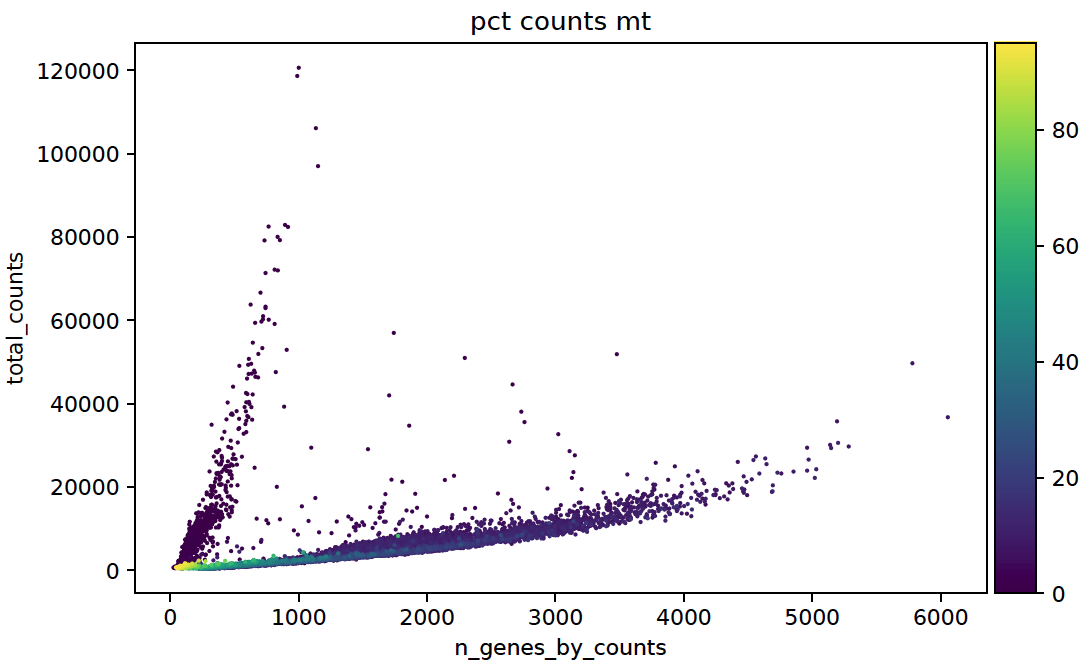
Visualize informative QC metrics and determine proper cutoffs:
for key in ['n_genes_by_counts','total_counts','pct_counts_mt']:
    sc.pl.violin(adata,key,jitter=0.4)
    plt.savefig('qc_violin_{}.pdf'.format(key),bbox_inches='tight')
    plt.close()

sc.pl.scatter(adata,x='n_genes_by_counts',y='total_counts',color='pct_counts_mt')
plt.savefig('qc_scatter.pdf',bbox_inches='tight')
plt.close()
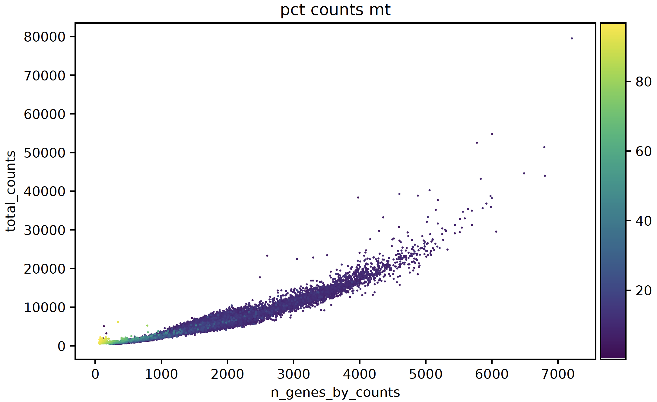
Then filter out the cells whose min_genes = 300, min_counts = 500, mt > 20%. There will be 11,022 cells left:
sc.pp.filter_cells(adata, min_genes=300)
sc.pp.filter_cells(adata, min_counts=500)
adata = adata[adata.obs.pct_counts_mt < 20, :]
print(adata)  # 11022 × 33538
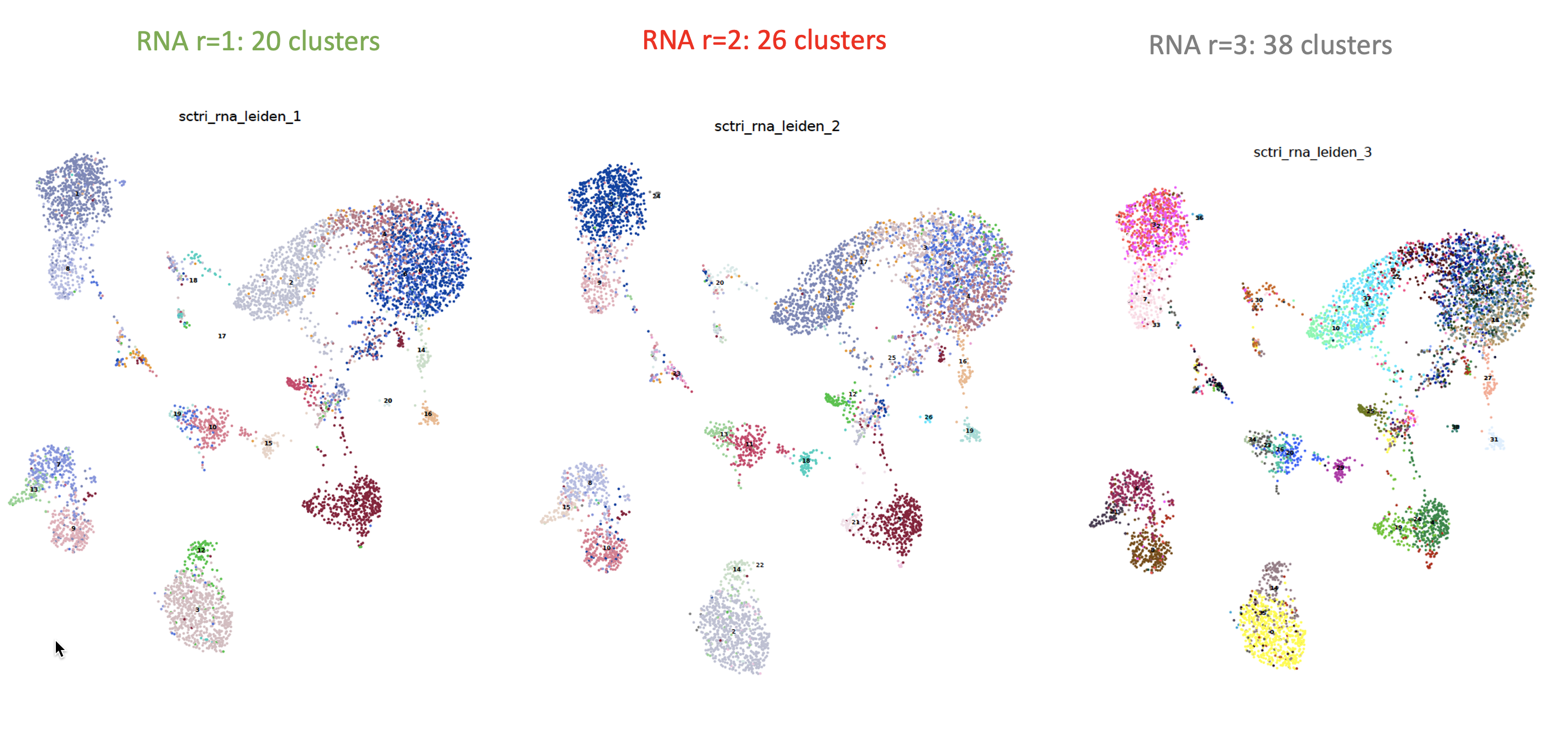
Then use the scTriangulate wrapper function to obtain the Leiden clustering results at different resolutions (r=1,2,3), specifically, we chose the number of PCs to be 50, and the highly variable genes to be 3000:
adata = scanpy_recipe(adata,is_log=False,resolutions=[1,2,3],pca_n_comps=50,n_top_genes=3000)
After running this command, you will populate three columns in adata.obs, namely, sctri_rna_leiden_1, sctri_rna_leiden_2, sctri_rna_leiden_3.
Also an h5ad file named adata_after_scanpy_recipe_rna_1_2_3_umap_True.h5ad will be automatically saved to the current directory so that there is no need to re-run this
pre-processing step again. Now let’s visualize these results:
umap_dual_view_save(adata,cols=['sctri_rna_leiden_1','sctri_rna_leiden_2','sctri_rna_leiden_3'])
# three umaps will be saved to your current directory.
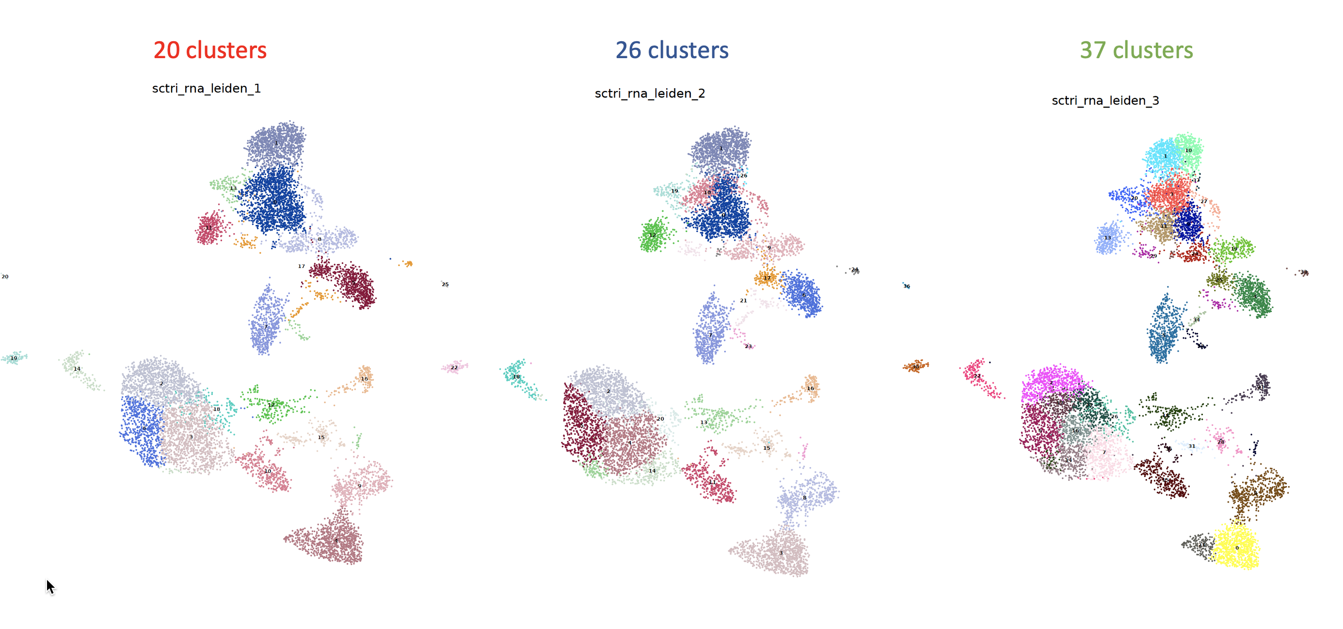
As you can see, different resolutions lead to various numbers of clusters, and it is clear that certain regions are sub-divided into sub-clusters associated with the higher resolution clustering. However, we don’t know whether these sub-populations are initially valid. Here scTriangulate will scan each of the clusters at each resolution, and mix-and-match different solutions to achieve a reconciled result.
Running scTriangulate
Default lazy run
Running scTriangulate can be as simple as two steps. We first instantiate the ScTriangulate object, then call the lazy_run class function which will
perform all of the downstream steps automatically:
adata = sc.read('adata_after_scanpy_recipe_rna_1_2_3_umap_True.h5ad')
sctri = ScTriangulate(dir='./output',adata=adata,query=['sctri_rna_leiden_1','sctri_rna_leiden_2','sctri_rna_leiden_3'])
sctri.lazy_run(assess_pruned=False,viewer_cluster=False,viewer_heterogeneity=False)  # done!!!
We first instantiate ScTriangulate object by specifying:
dir, where do all the intermediate and final results/plots will be saved to?adata, the adata that we want to start with.query, a list that contains all the annotations that we want to triangulate.
The dir doesn’t need to be an existing folder, the program will automatically create one if not present. More information about instantiation can be
found in the API __init__().
assess_pruned which will automatically assess the stability of the final defined cluster as well, generate the cluster viewer and heterogeneity viewer. Other
two arguments will automatically generate static HTML viewers. By default, we set them as False as the main purpose is to get scTriangulate clusters and stability.
You can switch them to True.
Note
However for the purpose of instructing user how to understand this tool, we are going to run it step-by-step to let the user get a sense of how the program works. We will refer to this as a Manual Run.
Manual Run
Step 1: Compute Metrics
The first step of running scTriangulate is to determine the biologically meaningful metrics for each cluster in each resolution. By default, scTriangulate will
use reassign score, TFIDF10 score, TFIDF5 score and SCCAF score to measure the robustness and stability of each cluster, the metrics can be modified
through sctri.metrics attribute list:
adata = sc.read('adata_after_scanpy_recipe_rna_1_2_3_umap_True.h5ad')
sctri = ScTriangulate(dir='./output',adata=adata,query=['sctri_rna_leiden_1','sctri_rna_leiden_2','sctri_rna_leiden_3'])
sctri.compute_metrics(parallel=True)
sctri.serialize('break_point_after_metrics.p')   # save it for next step
After this step, 3 * 4 = 12 columns will be added to the sctri.adata.obs dataframe. 3 = 3 resolutions, 4 = 4 metrics.
Those columns store the metrics we just calculated, the first 10 rows are shown below.
n_genes_by_counts |
total_counts |
total_counts_mt |
pct_counts_mt |
n_genes |
n_counts |
sctri_rna_leiden_1 |
sctri_rna_leiden_2 |
sctri_rna_leiden_3 |
doublet_scores |
||||||||||||||||
|---|---|---|---|---|---|---|---|---|---|---|---|---|---|---|---|---|---|---|---|---|---|---|---|---|---|
AAACCCAAGCGCCCAT-1 |
1087 |
2204.0 |
52.0 |
2.3593466 |
1087 |
2204.0 |
0 |
0 |
20 |
0.06075768406004289 |
0.8950276243093923 |
0.3439838075846785 |
0.9251533742331288 |
0.10092147725346746 |
0.37130280304671465 |
0.8042789223454834 |
0.3507859300918892 |
0.8890649762282092 |
0.10148899088645824 |
0.3805522921317833 |
0.704225352112676 |
0.4331249394858995 |
0.616822429906542 |
0.06823584435065695 |
0.5248428314538921 |
AAACCCAAGGTTCCGC-1 |
4200 |
20090.0 |
1324.0 |
6.5903435 |
4200 |
20090.0 |
14 |
18 |
22 |
0.032894736842105275 |
0.8297872340425532 |
0.8158574236335182 |
0.8617021276595744 |
0.06828310525665475 |
0.8788859218463015 |
0.9056603773584906 |
0.8757826138745951 |
0.9375 |
0.0669894608659765 |
1.0037564111504598 |
0.9005847953216374 |
0.8539603438702356 |
0.8470588235294118 |
0.0675555298114107 |
0.9552786801551147 |
AAACCCACAGAGTTGG-1 |
1836 |
5884.0 |
633.0 |
10.757988 |
1836 |
5884.0 |
2 |
2 |
2 |
0.05390835579514825 |
0.7060869565217391 |
0.4181291163421069 |
0.8104347826086956 |
0.07300475660048267 |
0.42582579367389656 |
0.6565853658536586 |
0.4078403118313299 |
0.787109375 |
0.07208010563020643 |
0.4239485989320037 |
0.6717791411042945 |
0.42090114511950677 |
0.7760736196319018 |
0.06426933099136449 |
0.4266449489575865 |
AAACCCACAGGTATGG-1 |
2216 |
5530.0 |
434.0 |
7.848101 |
2216 |
5530.0 |
7 |
7 |
5 |
0.008906882591093117 |
0.9783783783783784 |
0.7868703149865569 |
0.9820143884892086 |
0.034403601185809866 |
0.8771728968728391 |
0.9495495495495495 |
0.7868703149865569 |
0.9855595667870036 |
0.034403601185809866 |
0.8771728968728391 |
0.9207207207207208 |
0.7868703149865569 |
0.9820143884892086 |
0.034403601185809866 |
0.8771728968728391 |
AAACCCACATAGTCAC-1 |
1615 |
5106.0 |
553.0 |
10.830396 |
1615 |
5106.0 |
4 |
3 |
0 |
0.025075225677031094 |
0.9898682877406282 |
0.6648462514443869 |
0.9817813765182186 |
0.029651745213786315 |
0.7176015036667331 |
0.9916492693110647 |
0.6692931115772808 |
0.9770354906054279 |
0.02911431201925055 |
0.7193190390843421 |
0.9414758269720102 |
0.6523547740200044 |
0.9567430025445293 |
0.029681243164883617 |
0.7248931329792404 |
AAACCCACATCCAATG-1 |
1800 |
4572.0 |
411.0 |
8.989501 |
1800 |
4572.0 |
7 |
7 |
5 |
0.07363420427553445 |
0.9783783783783784 |
0.7868703149865569 |
0.9820143884892086 |
0.034403601185809866 |
0.8771728968728391 |
0.9495495495495495 |
0.7868703149865569 |
0.9855595667870036 |
0.034403601185809866 |
0.8771728968728391 |
0.9207207207207208 |
0.7868703149865569 |
0.9820143884892086 |
0.034403601185809866 |
0.8771728968728391 |
AAACCCAGTGGCTACC-1 |
1965 |
6702.0 |
424.0 |
6.32647 |
1965 |
6702.0 |
0 |
0 |
3 |
0.06849315068493152 |
0.8950276243093923 |
0.3439838075846785 |
0.9251533742331288 |
0.10092147725346746 |
0.37130280304671465 |
0.8042789223454834 |
0.3507859300918892 |
0.8890649762282092 |
0.10148899088645824 |
0.3805522921317833 |
0.790625 |
0.3736026863699238 |
0.64375 |
0.10099172212080179 |
0.40115765301328327 |
AAACCCATCCCGAGAC-1 |
1960 |
7092.0 |
545.0 |
7.6847153 |
1960 |
7092.0 |
0 |
0 |
3 |
0.104390243902439 |
0.8950276243093923 |
0.3439838075846785 |
0.9251533742331288 |
0.10092147725346746 |
0.37130280304671465 |
0.8042789223454834 |
0.3507859300918892 |
0.8890649762282092 |
0.10148899088645824 |
0.3805522921317833 |
0.790625 |
0.3736026863699238 |
0.64375 |
0.10099172212080179 |
0.40115765301328327 |
AAACCCATCTGGCCGA-1 |
1695 |
5370.0 |
571.0 |
10.633146 |
1695 |
5370.0 |
8 |
9 |
9 |
0.25563909774436094 |
0.7735849056603774 |
0.4140609851013919 |
0.907563025210084 |
0.13099806496107133 |
0.49547402236082677 |
0.7281553398058253 |
0.46148281492953686 |
0.8883495145631068 |
0.1427853920941894 |
0.5486776444570318 |
0.767590618336887 |
0.34400131931724975 |
0.7435897435897436 |
0.11643270856376918 |
0.3644349082676911 |
Step 2: Compute Shapley
The second step is to use the calculated metrics, and assess which annotation/cluster is the best for each single cell. So the program iterates through each row,
representing a single cell, retrieves all the metrics associated with each cluster, and calculates a Shapley value for each cluster (in this case, each single cell has
three conflicting clusters). Then the program will assign the cell to the “winning” cluster amongst all solutions. We refer the resultant cluster assignment as
the raw cluster result:
sctri = ScTriangulate.deserialize('output/break_point_after_metrics.p')
sctri.compute_shapley(parallel=True)
sctri.serialize('break_point_after_shapley.p')
After this step, 3 + 1 + 1 + 1 columns will be added to the sctri.adata.obs. They are the 3 columns corresponding to the Shapley value for each annotation, plus
one column named ‘final_annotation’ storing which annotation is the winner for each cell, and the column ‘raw’ contains raw clusters which are basically annotation
names and cluster names but concatenated by the @ symbol. The last added column is the ‘prefix’, which is just a concatenation of the original cluster and the current raw cluster.
n_genes_by_counts |
total_counts |
total_counts_mt |
pct_counts_mt |
n_genes |
n_counts |
sctri_rna_leiden_1 |
sctri_rna_leiden_2 |
sctri_rna_leiden_3 |
doublet_scores |
final_annotation |
sctri_rna_leiden_1_shapley |
sctri_rna_leiden_2_shapley |
sctri_rna_leiden_3_shapley |
raw |
prefixed |
||||||||||||||||
|---|---|---|---|---|---|---|---|---|---|---|---|---|---|---|---|---|---|---|---|---|---|---|---|---|---|---|---|---|---|---|---|
AAACCCAAGCGCCCAT-1 |
1087 |
2204.0 |
52.0 |
2.3593466 |
1087 |
2204.0 |
0 |
0 |
20 |
0.06075768406004289 |
0.8937998772252916 |
0.3439838075846785 |
0.9251533742331288 |
0.10092147725346746 |
0.37130280304671465 |
0.8050713153724247 |
0.3507859300918892 |
0.8890649762282092 |
0.10148899088645824 |
0.3805522921317833 |
0.6995305164319249 |
0.4331249394858995 |
0.616822429906542 |
0.06823584435065695 |
0.5248428314538921 |
sctri_rna_leiden_1 |
4.0 |
1.3333333333333333 |
3.333333333333333 |
sctri_rna_leiden_1@0 |
sctri_rna_leiden_1@0|sctri_rna_leiden_1@0 |
AAACCCAAGGTTCCGC-1 |
4200 |
20090.0 |
1324.0 |
6.5903435 |
4200 |
20090.0 |
14 |
18 |
22 |
0.032894736842105275 |
0.8297872340425532 |
0.8158574236335182 |
0.8617021276595744 |
0.06828310525665475 |
0.8788859218463015 |
0.9056603773584906 |
0.8757826138745951 |
0.9375 |
0.0669894608659765 |
1.0037564111504598 |
0.9005847953216374 |
0.8539603438702356 |
0.8470588235294118 |
0.0675555298114107 |
0.9552786801551147 |
sctri_rna_leiden_2 |
0.3333333333333333 |
6.666666666666666 |
2.333333333333333 |
sctri_rna_leiden_1@14|sctri_rna_leiden_2@18 |
|
AAACCCACAGAGTTGG-1 |
1836 |
5884.0 |
633.0 |
10.757988 |
1836 |
5884.0 |
2 |
2 |
2 |
0.05390835579514825 |
0.7095652173913043 |
0.4181291163421069 |
0.8104347826086956 |
0.07300475660048267 |
0.42582579367389656 |
0.6780487804878049 |
0.4078403118313299 |
0.787109375 |
0.07208010563020643 |
0.4239485989320037 |
0.6809815950920245 |
0.42090114511950677 |
0.7760736196319018 |
0.06426933099136449 |
0.4266449489575865 |
sctri_rna_leiden_1 |
6.666666666666666 |
2.333333333333333 |
3.6666666666666665 |
sctri_rna_leiden_1@2 |
sctri_rna_leiden_1@2|sctri_rna_leiden_1@2 |
AAACCCACAGGTATGG-1 |
2216 |
5530.0 |
434.0 |
7.848101 |
2216 |
5530.0 |
7 |
7 |
5 |
0.008906882591093117 |
0.9783783783783784 |
0.7868703149865569 |
0.9820143884892086 |
0.034403601185809866 |
0.8771728968728391 |
0.9477477477477477 |
0.7868703149865569 |
0.9855595667870036 |
0.034403601185809866 |
0.8771728968728391 |
0.918918918918919 |
0.7868703149865569 |
0.9820143884892086 |
0.034403601185809866 |
0.8771728968728391 |
sctri_rna_leiden_1 |
6.666666666666666 |
5.333333333333333 |
5.0 |
sctri_rna_leiden_1@7 |
sctri_rna_leiden_1@7|sctri_rna_leiden_1@7 |
AAACCCACATAGTCAC-1 |
1615 |
5106.0 |
553.0 |
10.830396 |
1615 |
5106.0 |
4 |
3 |
0 |
0.025075225677031094 |
0.9898682877406282 |
0.6648462514443869 |
0.9817813765182186 |
0.029651745213786315 |
0.7176015036667331 |
0.9916492693110647 |
0.6692931115772808 |
0.9770354906054279 |
0.02911431201925055 |
0.7193190390843421 |
0.9402035623409669 |
0.6523547740200044 |
0.9567430025445293 |
0.029681243164883617 |
0.7248931329792404 |
sctri_rna_leiden_2 |
6.666666666666666 |
6.666666666666666 |
1.6666666666666665 |
sctri_rna_leiden_2@3 |
sctri_rna_leiden_1@4|sctri_rna_leiden_2@3 |
AAACCCACATCCAATG-1 |
1800 |
4572.0 |
411.0 |
8.989501 |
1800 |
4572.0 |
7 |
7 |
5 |
0.07363420427553445 |
0.9783783783783784 |
0.7868703149865569 |
0.9820143884892086 |
0.034403601185809866 |
0.8771728968728391 |
0.9477477477477477 |
0.7868703149865569 |
0.9855595667870036 |
0.034403601185809866 |
0.8771728968728391 |
0.918918918918919 |
0.7868703149865569 |
0.9820143884892086 |
0.034403601185809866 |
0.8771728968728391 |
sctri_rna_leiden_1 |
6.666666666666666 |
5.333333333333333 |
5.0 |
sctri_rna_leiden_1@7 |
sctri_rna_leiden_1@7|sctri_rna_leiden_1@7 |
AAACCCAGTGGCTACC-1 |
1965 |
6702.0 |
424.0 |
6.32647 |
1965 |
6702.0 |
0 |
0 |
3 |
0.06849315068493152 |
0.8937998772252916 |
0.3439838075846785 |
0.9251533742331288 |
0.10092147725346746 |
0.37130280304671465 |
0.8050713153724247 |
0.3507859300918892 |
0.8890649762282092 |
0.10148899088645824 |
0.3805522921317833 |
0.7859375 |
0.3736026863699238 |
0.64375 |
0.10099172212080179 |
0.40115765301328327 |
sctri_rna_leiden_1 |
4.0 |
1.3333333333333333 |
3.333333333333333 |
sctri_rna_leiden_1@0 |
sctri_rna_leiden_1@0|sctri_rna_leiden_1@0 |
AAACCCATCCCGAGAC-1 |
1960 |
7092.0 |
545.0 |
7.6847153 |
1960 |
7092.0 |
0 |
0 |
3 |
0.104390243902439 |
0.8937998772252916 |
0.3439838075846785 |
0.9251533742331288 |
0.10092147725346746 |
0.37130280304671465 |
0.8050713153724247 |
0.3507859300918892 |
0.8890649762282092 |
0.10148899088645824 |
0.3805522921317833 |
0.7859375 |
0.3736026863699238 |
0.64375 |
0.10099172212080179 |
0.40115765301328327 |
sctri_rna_leiden_1 |
4.0 |
1.3333333333333333 |
3.333333333333333 |
sctri_rna_leiden_1@0 |
sctri_rna_leiden_1@0|sctri_rna_leiden_1@0 |
AAACCCATCTGGCCGA-1 |
1695 |
5370.0 |
571.0 |
10.633146 |
1695 |
5370.0 |
8 |
9 |
9 |
0.25563909774436094 |
0.7672955974842768 |
0.4140609851013919 |
0.907563025210084 |
0.13099806496107133 |
0.49547402236082677 |
0.7330097087378641 |
0.46148281492953686 |
0.8883495145631068 |
0.1427853920941894 |
0.5486776444570318 |
0.7633262260127932 |
0.34400131931724975 |
0.7435897435897436 |
0.11643270856376918 |
0.3644349082676911 |
sctri_rna_leiden_1 |
4.0 |
3.6666666666666665 |
1.6666666666666665 |
sctri_rna_leiden_1@8 |
sctri_rna_leiden_1@8|sctri_rna_leiden_1@8 |
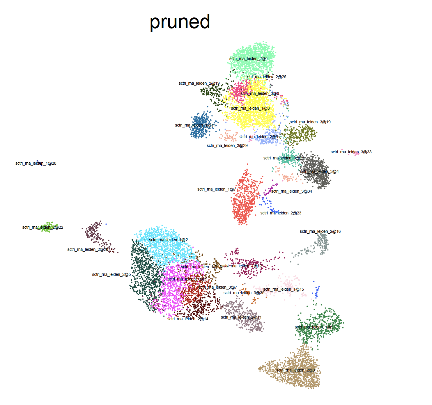
Step 3: Prune the results
This step is used to prune the raw result. In many cases, the raw results will contain clusters which represent a small fraction of cells relative to
the original parental cluster. In these cases, it can be advantageous to remove these more speculative results by filtering these out and reclassify
all cells against the remaining clusters. First, we evaluate the robustness of the raw clustering results using the same set of stability metrics and
and add the relatively unstable clusters to invalid category, based on the proportion of cells in the raw results versus the source annotations.
This will be defiend by win_fraction < 0.25 by default, meaning if a cluster originally has 100 cells, but has <25 cells left. The cells in these
unstable invalid clusters will be reassigned to its nearest neightbor’s cluster label. After this step, we have pruned reusult:
sctri = ScTriangulate.deserialize('output/break_point_after_shapley.p')
sctri.prune_result()
sctri.serialize('break_point_after_prune.p')
A column named “pruned” will be added, also a “confidence” column stores the confidence the software has to represent this cluster.
n_genes_by_counts |
total_counts |
total_counts_mt |
pct_counts_mt |
n_genes |
n_counts |
sctri_rna_leiden_1 |
sctri_rna_leiden_2 |
sctri_rna_leiden_3 |
doublet_scores |
final_annotation |
sctri_rna_leiden_1_shapley |
sctri_rna_leiden_2_shapley |
sctri_rna_leiden_3_shapley |
raw |
prefixed |
pruned |
confidence |
ori |
||||||||||||||||||||||||||
|---|---|---|---|---|---|---|---|---|---|---|---|---|---|---|---|---|---|---|---|---|---|---|---|---|---|---|---|---|---|---|---|---|---|---|---|---|---|---|---|---|---|---|---|---|
AAACCCAAGCGCCCAT-1 |
1087 |
2204.0 |
52.0 |
2.3593466 |
1087 |
2204.0 |
0 |
0 |
20 |
0.06075768406004289 |
0.8937998772252916 |
0.3439838075846785 |
0.9251533742331288 |
0.10092147725346746 |
0.37130280304671465 |
0.8050713153724247 |
0.3507859300918892 |
0.8890649762282092 |
0.10148899088645824 |
0.3805522921317833 |
0.6995305164319249 |
0.4331249394858995 |
0.616822429906542 |
0.06823584435065695 |
0.5248428314538921 |
sctri_rna_leiden_1 |
4.0 |
1.3333333333333333 |
3.333333333333333 |
sctri_rna_leiden_1@0 |
sctri_rna_leiden_1@0|sctri_rna_leiden_1@0 |
0.6856508875739645 |
0.3422339406894759 |
0.8668639053254438 |
0.09982013932055393 |
0.37524819649429547 |
sctri_rna_leiden_1@0 |
0.8299570288520565 |
0 |
0.7318681318681318 |
0.34087432957319 |
0.890190336749634 |
0.09965020294622279 |
0.372858462455373 |
AAACCCAAGGTTCCGC-1 |
4200 |
20090.0 |
1324.0 |
6.5903435 |
4200 |
20090.0 |
14 |
18 |
22 |
0.032894736842105275 |
0.8297872340425532 |
0.8158574236335182 |
0.8617021276595744 |
0.06828310525665475 |
0.8788859218463015 |
0.9056603773584906 |
0.8757826138745951 |
0.9375 |
0.0669894608659765 |
1.0037564111504598 |
0.9005847953216374 |
0.8539603438702356 |
0.8470588235294118 |
0.0675555298114107 |
0.9552786801551147 |
sctri_rna_leiden_2 |
0.3333333333333333 |
6.666666666666666 |
2.333333333333333 |
sctri_rna_leiden_1@14|sctri_rna_leiden_2@18 |
0.8050314465408805 |
0.8767835124228538 |
0.9625 |
0.0669894608659765 |
1.0036722009000825 |
1.0 |
1 |
0.9259259259259259 |
0.8715118012431851 |
0.9382716049382716 |
0.06659199654812879 |
0.9851686771624536 |
||
AAACCCACAGAGTTGG-1 |
1836 |
5884.0 |
633.0 |
10.757988 |
1836 |
5884.0 |
2 |
2 |
2 |
0.05390835579514825 |
0.7095652173913043 |
0.4181291163421069 |
0.8104347826086956 |
0.07300475660048267 |
0.42582579367389656 |
0.6780487804878049 |
0.4078403118313299 |
0.787109375 |
0.07208010563020643 |
0.4239485989320037 |
0.6809815950920245 |
0.42090114511950677 |
0.7760736196319018 |
0.06426933099136449 |
0.4266449489575865 |
sctri_rna_leiden_1 |
6.666666666666666 |
2.333333333333333 |
3.6666666666666665 |
sctri_rna_leiden_1@2 |
sctri_rna_leiden_1@2|sctri_rna_leiden_1@2 |
0.6542338709677419 |
0.40788362684536184 |
0.7701612903225806 |
0.07158873082273735 |
0.4237630150366414 |
sctri_rna_leiden_1@2 |
0.8626086956521739 |
2 |
0.6700100300902708 |
0.4079180019195594 |
0.7831325301204819 |
0.07165279317880446 |
0.42336364967356116 |
AAACCCACAGGTATGG-1 |
2216 |
5530.0 |
434.0 |
7.848101 |
2216 |
5530.0 |
7 |
7 |
5 |
0.008906882591093117 |
0.9783783783783784 |
0.7868703149865569 |
0.9820143884892086 |
0.034403601185809866 |
0.8771728968728391 |
0.9477477477477477 |
0.7868703149865569 |
0.9855595667870036 |
0.034403601185809866 |
0.8771728968728391 |
0.918918918918919 |
0.7868703149865569 |
0.9820143884892086 |
0.034403601185809866 |
0.8771728968728391 |
sctri_rna_leiden_1 |
6.666666666666666 |
5.333333333333333 |
5.0 |
sctri_rna_leiden_1@7 |
sctri_rna_leiden_1@7|sctri_rna_leiden_1@7 |
0.9153153153153153 |
0.7867280231606432 |
0.9748201438848921 |
0.034403601185809866 |
0.8770345847482843 |
sctri_rna_leiden_1@7 |
1.0 |
3 |
0.9117117117117117 |
0.7868703149865569 |
0.9819494584837545 |
0.034403601185809866 |
0.8771728968728391 |
AAACCCACATAGTCAC-1 |
1615 |
5106.0 |
553.0 |
10.830396 |
1615 |
5106.0 |
4 |
3 |
0 |
0.025075225677031094 |
0.9898682877406282 |
0.6648462514443869 |
0.9817813765182186 |
0.029651745213786315 |
0.7176015036667331 |
0.9916492693110647 |
0.6692931115772808 |
0.9770354906054279 |
0.02911431201925055 |
0.7193190390843421 |
0.9402035623409669 |
0.6523547740200044 |
0.9567430025445293 |
0.029681243164883617 |
0.7248931329792404 |
sctri_rna_leiden_2 |
6.666666666666666 |
6.666666666666666 |
1.6666666666666665 |
sctri_rna_leiden_2@3 |
sctri_rna_leiden_1@4|sctri_rna_leiden_2@3 |
0.9102296450939458 |
0.6694248039875961 |
0.9874739039665971 |
0.02911431201925055 |
0.7191829641398122 |
sctri_rna_leiden_2@3 |
1.0 |
4 |
0.9898682877406282 |
0.6648462514443869 |
0.9837728194726166 |
0.029651745213786315 |
0.7176015036667331 |
AAACCCACATCCAATG-1 |
1800 |
4572.0 |
411.0 |
8.989501 |
1800 |
4572.0 |
7 |
7 |
5 |
0.07363420427553445 |
0.9783783783783784 |
0.7868703149865569 |
0.9820143884892086 |
0.034403601185809866 |
0.8771728968728391 |
0.9477477477477477 |
0.7868703149865569 |
0.9855595667870036 |
0.034403601185809866 |
0.8771728968728391 |
0.918918918918919 |
0.7868703149865569 |
0.9820143884892086 |
0.034403601185809866 |
0.8771728968728391 |
sctri_rna_leiden_1 |
6.666666666666666 |
5.333333333333333 |
5.0 |
sctri_rna_leiden_1@7 |
sctri_rna_leiden_1@7|sctri_rna_leiden_1@7 |
0.9153153153153153 |
0.7867280231606432 |
0.9748201438848921 |
0.034403601185809866 |
0.8770345847482843 |
sctri_rna_leiden_1@7 |
1.0 |
5 |
0.9117117117117117 |
0.7868703149865569 |
0.9819494584837545 |
0.034403601185809866 |
0.8771728968728391 |
AAACCCAGTGGCTACC-1 |
1965 |
6702.0 |
424.0 |
6.32647 |
1965 |
6702.0 |
0 |
0 |
3 |
0.06849315068493152 |
0.8937998772252916 |
0.3439838075846785 |
0.9251533742331288 |
0.10092147725346746 |
0.37130280304671465 |
0.8050713153724247 |
0.3507859300918892 |
0.8890649762282092 |
0.10148899088645824 |
0.3805522921317833 |
0.7859375 |
0.3736026863699238 |
0.64375 |
0.10099172212080179 |
0.40115765301328327 |
sctri_rna_leiden_1 |
4.0 |
1.3333333333333333 |
3.333333333333333 |
sctri_rna_leiden_1@0 |
sctri_rna_leiden_1@0|sctri_rna_leiden_1@0 |
0.6856508875739645 |
0.3422339406894759 |
0.8668639053254438 |
0.09982013932055393 |
0.37524819649429547 |
sctri_rna_leiden_1@0 |
0.8299570288520565 |
6 |
0.7318681318681318 |
0.34087432957319 |
0.890190336749634 |
0.09965020294622279 |
0.372858462455373 |
AAACCCATCCCGAGAC-1 |
1960 |
7092.0 |
545.0 |
7.6847153 |
1960 |
7092.0 |
0 |
0 |
3 |
0.104390243902439 |
0.8937998772252916 |
0.3439838075846785 |
0.9251533742331288 |
0.10092147725346746 |
0.37130280304671465 |
0.8050713153724247 |
0.3507859300918892 |
0.8890649762282092 |
0.10148899088645824 |
0.3805522921317833 |
0.7859375 |
0.3736026863699238 |
0.64375 |
0.10099172212080179 |
0.40115765301328327 |
sctri_rna_leiden_1 |
4.0 |
1.3333333333333333 |
3.333333333333333 |
sctri_rna_leiden_1@0 |
sctri_rna_leiden_1@0|sctri_rna_leiden_1@0 |
0.6856508875739645 |
0.3422339406894759 |
0.8668639053254438 |
0.09982013932055393 |
0.37524819649429547 |
sctri_rna_leiden_1@0 |
0.8299570288520565 |
7 |
0.7318681318681318 |
0.34087432957319 |
0.890190336749634 |
0.09965020294622279 |
0.372858462455373 |
AAACCCATCTGGCCGA-1 |
1695 |
5370.0 |
571.0 |
10.633146 |
1695 |
5370.0 |
8 |
9 |
9 |
0.25563909774436094 |
0.7672955974842768 |
0.4140609851013919 |
0.907563025210084 |
0.13099806496107133 |
0.49547402236082677 |
0.7330097087378641 |
0.46148281492953686 |
0.8883495145631068 |
0.1427853920941894 |
0.5486776444570318 |
0.7633262260127932 |
0.34400131931724975 |
0.7435897435897436 |
0.11643270856376918 |
0.3644349082676911 |
sctri_rna_leiden_1 |
4.0 |
3.6666666666666665 |
1.6666666666666665 |
sctri_rna_leiden_1@8 |
sctri_rna_leiden_1@8|sctri_rna_leiden_2@9 |
0.8125 |
0.26366270719185436 |
0.5 |
0.07300331728524727 |
0.3589422599550743 |
sctri_rna_leiden_2@9 |
0.13417190775681342 |
8 |
0.8958333333333334 |
0.3804105780430053 |
0.5625 |
0.1860030766024984 |
0.4289774942532307 |
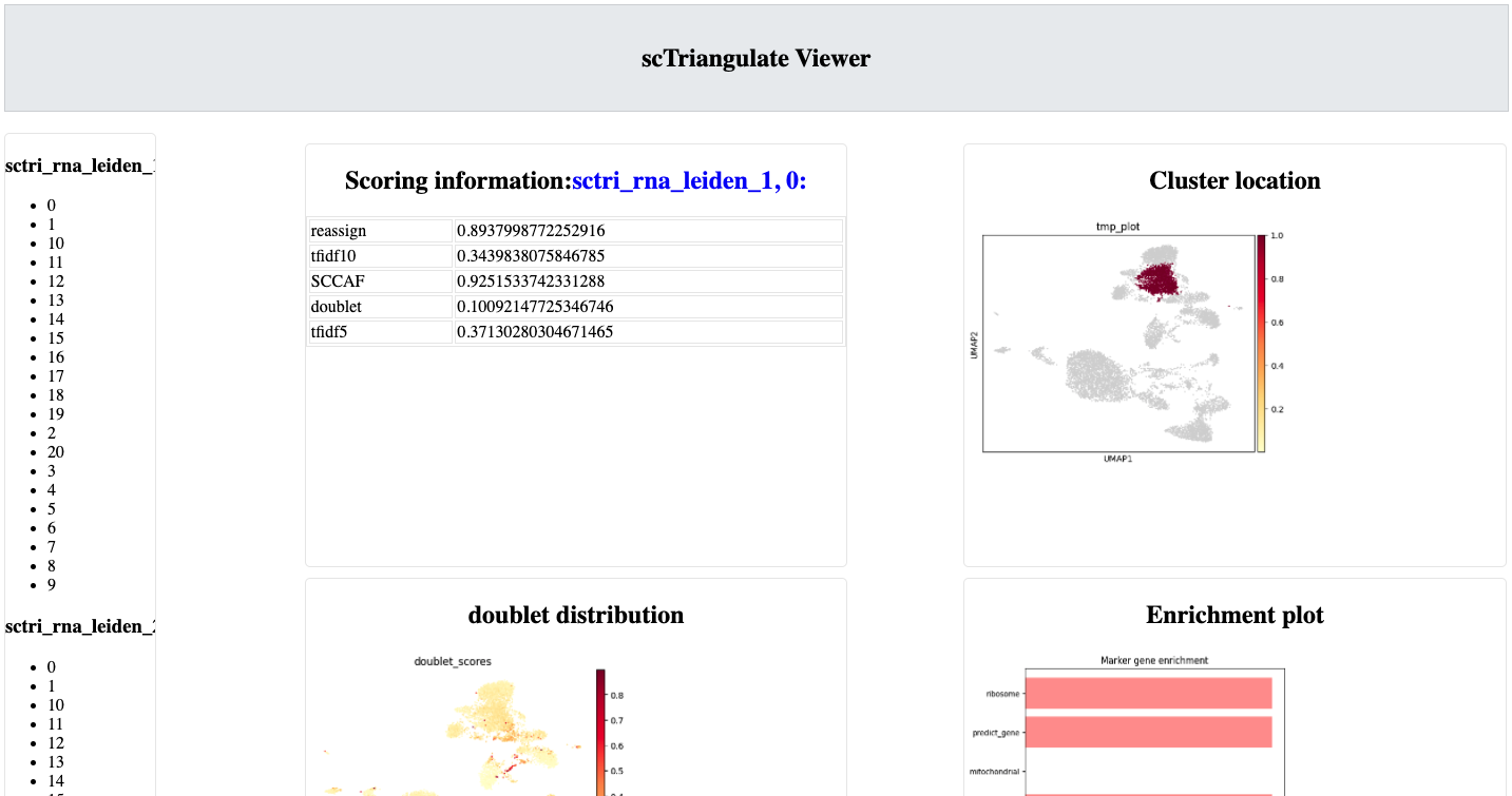
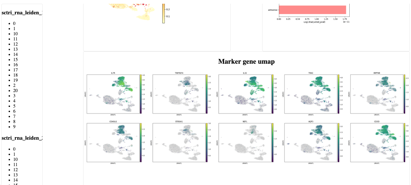
Step 4: Building the Viewer
We provide an automatically generated html archive, called the scTriangulate viewer, to allow users to dynamically toggle between different clusters, including the robustness of each cluster from each annotation (cluster viewer). In addtion, it enables the inspection of further heterogeneity that might not have been captured by a single annotation (hetergeneity viewer). The logic of the following functions are simple. We first build the html pages, then we generate the figures that the html pages will need for proper rendering:
sctri = ScTriangulate.deserialize('output/break_point_after_prune.p')
sctri.viewer_cluster_feature_html()
sctri.viewer_cluster_feature_figure(parallel=False,select_keys=['sctri_rna_leiden_1','pruned'])
sctri.viewer_heterogeneity_html(key='sctri_rna_leiden_1')
sctri.viewer_heterogeneity_figure(key='sctri_rna_leiden_1')
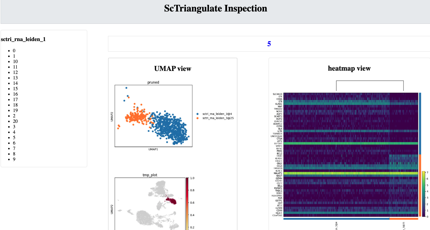
Inspect the results
Now we start to look at the scTriangulate results,
Comparison with Azimuth mapping
Azimuth leverages > 200 ADTs to delineate the major cell populations in PBMCs, which can serve as a silver standard. First we obtain the Azimuth mapping results using the h5ad object after we performed QC. Azimuth predction results can be downloaded from (http://altanalyze.org/scTriangulate/scRNASeq/azimuth_pred.tsv):
sctri = ScTriangulate.deserialize('output/break_point_after_prune.p')
add_azimuth(sctri.adata,'azimuth_pred.tsv')
for col in ['azimuth','pruned','final_annotation']:
    sctri.plot_umap(col,'category')
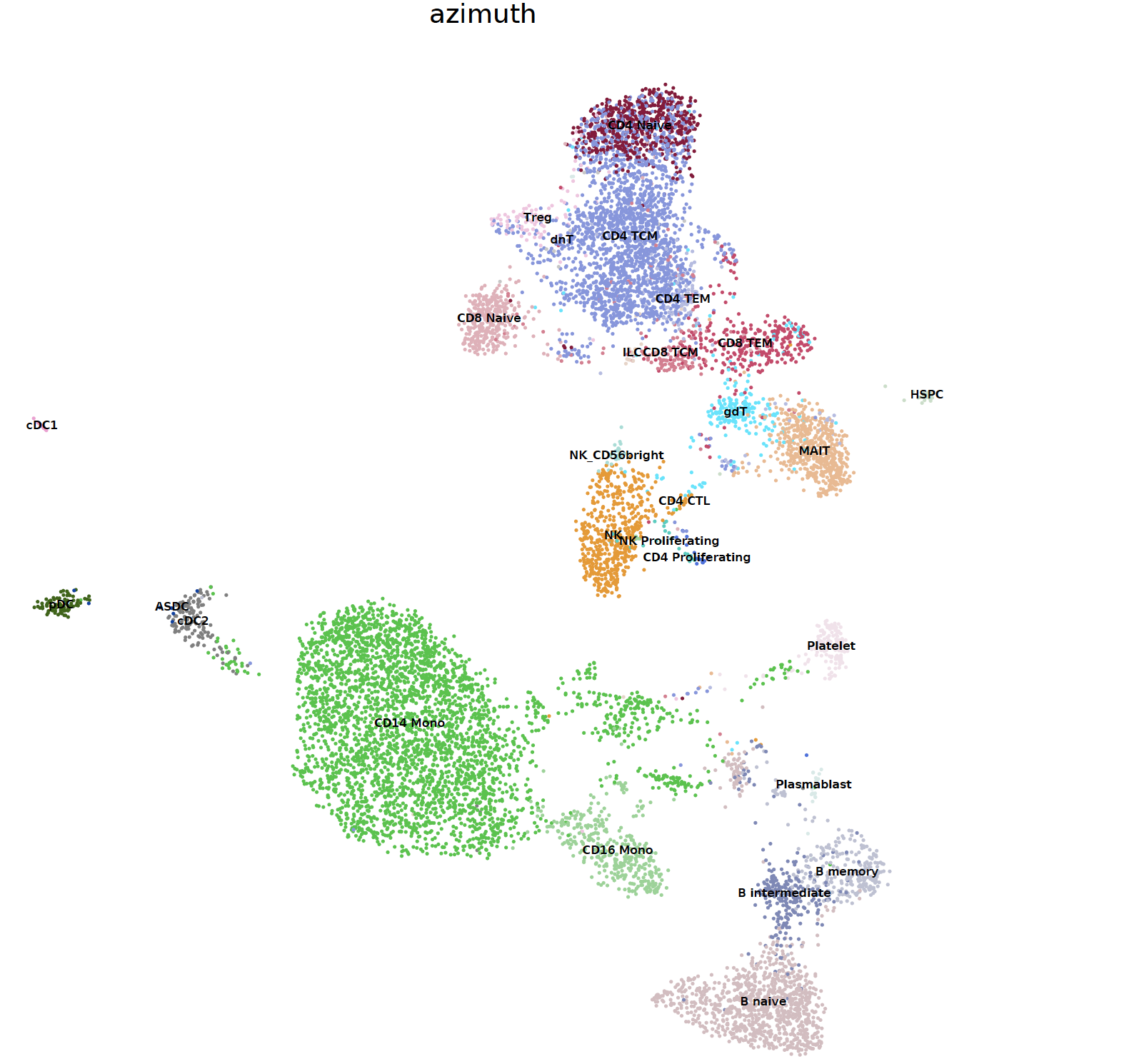
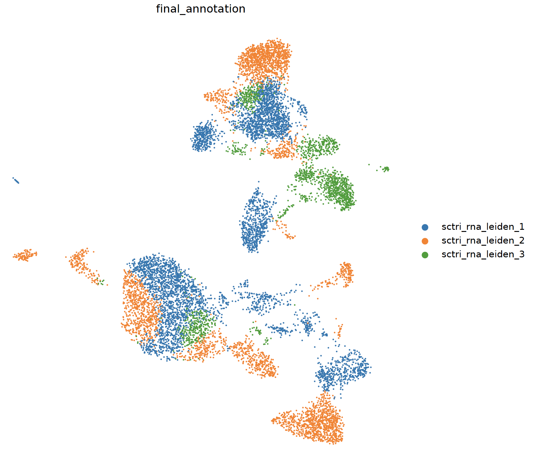
As you can see, scTriangulate can mix-and-match different resolutions, shown in the final_annotation column, and the merged final results have good
agreement with Azimuth.
Multi-modal workflow
In this example run, we are going to use a CITE-Seq dataset from human total nucleated cells (TNCs). This dataset contains 31 ADTs and in toal 8,491 cells. It is a common practice to analyze and cluster based on each modality seperately, and then try to merge them result together. However, to reconcile the clustering differences are not a trivial tasks and it requires the simoutaneous consideration of both RNA gene expression and surface protein. Thankfully, scTriangulate can help us make the decision.
the dataset can be downloaded from the http://altanalyze.org/scTriangulate/CITESeq/TNC_r1-RNA-ADT.h5.
As a more general explanation of how scTriangulate can be used in multi-modal setting, we use a pictorial representation:
Load data and preprocessing
Load packages:
import pandas as pd
import numpy as np
import os,sys
import scanpy as sc
from sctriangulate import *
from sctriangulate.preprocessing import *
Load the data:
adata = sc.read_10x_h5('28WM_ND19-341__TNC-RNA-ADT.h5',gex_only=False)
adata_rna = adata[:,adata.var['feature_types']=='Gene Expression']
adata_adt = adata[:,adata.var['feature_types']=='Antibody Capture']  # 8491

adata_rna.var_names_make_unique()
adata_adt.var_names_make_unique()
QC on RNA:
adata_rna.var['mt'] = adata_rna.var_names.str.startswith('MT-')
sc.pp.calculate_qc_metrics(adata_rna, qc_vars=['mt'], percent_top=None, log1p=False, inplace=True)

for key in ['n_genes_by_counts','total_counts','pct_counts_mt']:
    sc.pl.violin(adata_rna,key,jitter=0.4)
    plt.savefig('qc_rna_violin_{}.pdf'.format(key),bbox_inches='tight')
    plt.close()

sc.pl.scatter(adata_rna,x='n_genes_by_counts',y='total_counts',color='pct_counts_mt')
plt.savefig('qc_rna_scatter.pdf',bbox_inches='tight')
plt.close()
We filtered out the cells whose min_genes < 300, min_counts < 500, mt > 20%, there will be 6,406 cells kept:
sc.pp.filter_cells(adata_rna, min_genes=300)
sc.pp.filter_cells(adata_rna, min_counts=500)
adata_rna = adata_rna[adata_rna.obs.pct_counts_mt < 20, :]
adata_adt = adata_adt[adata_rna.obs_names,:]   # 6406
Perform unsupervised Leiden clustering on each of the modality, and then combined two adata objects:
adata_rna = scanpy_recipe(adata_rna,is_log=False,resolutions=[1,2,3],modality='rna',pca_n_comps=50)
adata_adt = scanpy_recipe(adata_adt,is_log=False,resolutions=[1,2,3],modality='adt',pca_n_comps=15)
adata_combine = concat_rna_and_other(adata_rna,adata_adt,umap='other',name='adt',prefix='AB_')
Running scTriangulate
Just use lazy_run() function, I have broken it down in the single_modality section:
sctri = ScTriangulate(dir='output',adata=adata_combine,add_metrics={},query=['sctri_adt_leiden_1','sctri_adt_leiden_2','sctri_adt_leiden_3','sctri_rna_leiden_1','sctri_rna_leiden_2','sctri_rna_leiden_3'])
sctri.lazy_run(assess_pruned=False,viewer_cluster=False,viewer_heterogeneity=False,added_metrics_kwargs=[])
All the intermediate results will be stored at ./output folder.
Inspect the results
scTriangulate allows the triangulation amongst diverse resolutions and modalities:
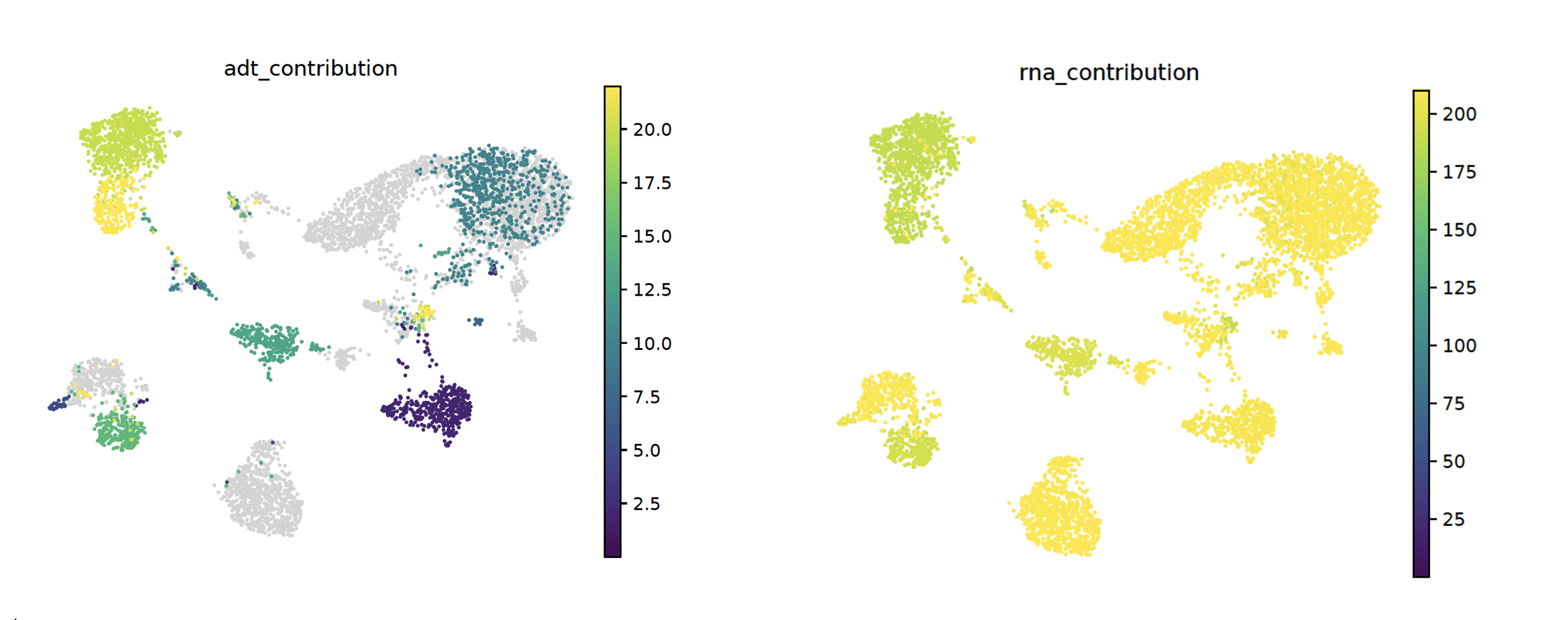
# get modality contributions
sctri = ScTriangulate.deserialize('output/after_pruned_assess.p')
sctri.modality_contributions()
for col in ['adt_contribution','rna_contribution']:
sctri.plot_umap(col,'continuous',umap_cmap='viridis')
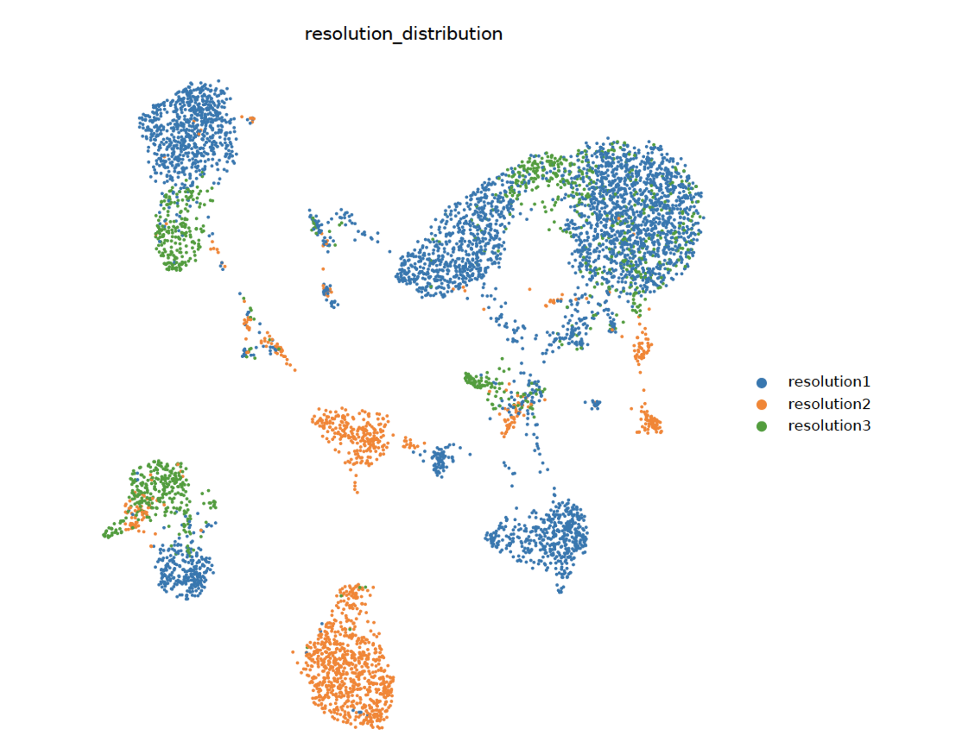
# get resolution distribution
col = []
for item in sctri.adata.obs['pruned']:
if 'leiden_1@' in item:
col.append('resolution1')
elif 'leiden_2@' in item:
col.append('resolution2')
elif 'leiden_3@' in item:
col.append('resolution3')
sctri.adata.obs['resolution_distribution'] = col
sctri.plot_umap('resolution_distribution','category')
scTriangulate can visualize the top markers in each cluster, example output see plot_multi_modal_feature_rank
sctri.plot_multi_modal_feature_rank(cluster='sctri_rna_leiden_3@6')
scTriangulate discovers new cell states from the ADT markers (CD56 high MAIT cell), supported by previous literature, azimuth prediction can be downloaded from (http://altanalyze.org/scTriangulate/CITESeq/azimuth_pred.tsv):
sctri = ScTriangulate.deserialize('output/after_pruned_assess.p')
add_azimuth(sctri.adata,'azimuth_pred.tsv')
sctri.adata.obs['dummy_key'] = np.full(sctri.adata.obs.shape[0],'dummy_cluster')
sctri.plot_heterogeneity('dummy_key','dummy_cluster','umap',col='azimuth',subset=['CD8 TEM','CD4 CTL','MAIT','dnT','CD8 Naive'])
sctri.plot_heterogeneity('dummy_key','dummy_cluster','umap',col='pruned',subset=['sctri_rna_leiden_3@6','sctri_rna_leiden_2@15','sctri_adt_leiden_3@37','sctri_adt_leiden_3@32','sctri_rna_leiden_1@9'])
sctri.plot_heterogeneity('dummy_key','dummy_cluster','single_gene',col='azimuth',subset=['CD8 TEM','CD4 CTL','MAIT','dnT','CD8 Naive'],single_gene='AB_CD56',umap_cmap='viridis')